Using ButterKnife in PSLab Android App

ButterKnife is an Android Library which is used for View injection and binding. Unlike Dagger, ButterKnife is limited to views whereas Dagger has a much broader utility and can be used for injection of anything like views, fragments etc. Being limited to views makes it much more simpler to use compared to dagger.

The need for using ButterKnife in our project PSLab Android was felt due to the fact binding views would be much more simpler in case of layouts like that of Oscilloscope Menu which has multiple views in the form of Textboxes, Checkboxes, Seekbars, Popups etc. Also, ButterKnife makes it possible to access the views outside the file in which they were declared. In this blog, the use of ButterKnife is limited to activities and fragments.

ButterKnife can used anywhere we would have otherwise used findViewById(). It helps in preventing code repetition while instantiating views in the layout. The ButterKnife blog has neatly listed all the possible uses of the library.

The added advantage of using Butterknife are-

  • The hassle of using Boilerplate code is not needed and the code volume is reduced significantly in some cases.
  • Setting up ButterKnife is quite easy as all it takes is adding one dependency to your gradle file.
  • It also has other features like Resource Binding (i.e binding String, Color, Drawable etc.).
  • Other uses like simplification of code while using buttons. For example, there is no need of using findViewById and setOnClickListener, simple annotation of the button ID with @OnClick does the task.

Using butterknife was essential for PSLab Android since for the views shown below which has too many elements, writing boilerplate code can be a very tedious task.

Using ButterKnife in activities

The PSLab App defines several activities like MainActivity, SplashActivity, ControlActivity etc. each of which consists of views that can be injected with ButterKnife.

After setting up ButterKnife by adding dependencies in gradle files, import these modules in every activity.

import butterknife.BindView;
import butterknife.ButterKnife;

Traditionally, views in Android are defined as follows using the ID defined in a layout file. For this findViewById is used to retrieve the widgets.

private NavigationView navigationView;
private DrawerLayout drawer;
private Toolbar toolbar;

navigationView = (NavigationView) findViewById(org.fossasia.pslab.R.id.nav_view);
drawer = (DrawerLayout) findViewById(org.fossasia.pslab.R.id.drawer_layout);
toolbar = (Toolbar) findViewById(org.fossasia.pslab.R.id.toolbar);

However, with the use of Butterknife, fields are annotated with @BindView and a View ID for finding and casting the view automatically in the layout files.
After the annotation, finding and casting of views ButterKnife.bind(this) is called to bind the views in the corresponding activity.

@BindView(R.id.nav_view) NavigationView navigationView;
@BindView(R.id.drawer_layout) DrawerLayout drawer;
@BindView(R.id.toolbar) Toolbar toolbar;
setContentView(R.layout.activity_main);
ButterKnife.bind(this);

Using ButterKnife in fragments

The PSLab Android App implements ApplicationFragment, DesignExperimentsFragment, HomeFragment etc., so ButterKnife for fragments is also used.

Using ButterKnife is fragments is slightly different from using it in activities as the binded views need to be destroyed on leaving the fragment as the fragments have different life cycle( Read about it here). For this an Unbinder needs to be defined to unbind the views before they are destroyed.

Quoting from the official documentation

When binding a fragment in OnCreateView, set the views to null in OnDestroyView. Butter Knife returns an Unbinder instance when you call bind to do this for you. Call its unbind method in the appropriate lifecycle callback.

So, an additional module of ButterKnife is imported

import butterknife.BindView;
import butterknife.ButterKnife;
import butterknife.Unbinder;

Similar as that of activities, the code below can be replaced by the corresponding ButterKnife code.

TextView tvDeviceStatus = (TextView)view.findViewById(org.fossasia.pslab.R.id.tv_device_status);
TextView tvVersion = (TextView)view.findViewById(org.fossasia.pslab.R.id.tv_device_version);
ImageView imgViewDeviceStatus = (ImageView)view.findViewById(org.fossasia.pslab.R.id.img_device_status);
@BindView(R.id.tv_device_status) TextView tvDeviceStatus;
@BindView(R.id.tv_device_version) TextView tvVersion;
@BindView(R.id.img_device_status) ImageView imgViewDeviceStatus;
private Unbinder unbinder;

Additionally, the unbinder object is used to store the returned Unbinder instance when ButterKnife.bind is called for Fragments.

unbinder = ButterKnife.bind(this,view);

Finally, the unbind method of unbinder is called while view is destroyed.

@Override public void onDestroyView() {
super.onDestroyView();
unbinder.unbind();
}

Continue ReadingUsing ButterKnife in PSLab Android App

Prototyping PSLab Android App using Invision

Often, while designing apps, we need planning and proper designing before actually building the apps. This is where mock-up tools and prototyping is useful. While designing user interfaces, the first step is usually creating mockups. Mockups give quite a good idea about the appearance of various layouts of the app. However, mockups are just still images and they don’t give a clue about the user experience of the app. This is where prototyping tools are useful. Prototyping helps to get an idea about the user experience without actually building the app.

Invision is an online prototyping service which was used for initial testing of the PSLab Android app. Some of pictures below are the screenshots of our prototype taken in Invision. Since, it supports collaboration among developers, it proves to be a very useful tool. 

  • Using Invision is quite simple. Visit the Invision website and sign up for an account.Before using invision for prototyping, the mockups of the UI layouts must be ready since Invision is simply meant for prototyping and not creating mockups. There are a lot of mock-up tools available online which are quite easy to use.
  • Create a new project on Invision. Select the project type – Prototype in this case followed by selecting the platform of the project i.e. Android, iOS etc.
  • Collaborators can be added to a project for working together.
    • After project creation and adding collaborators is done with, the mock-up screens can be uploaded to the project directory
    • Select any mock-up screen, the window below appears, there are a few modes available in the bottom navbar – Preview mode, Build mode, Comment mode, Inspect Mode and History Mode.
        • Preview Mode – View your screen and test the particular screen prototype.
        • Build Mode – Assign functionality to buttons, navbars, seek bars, check boxes etc. and other features like transitions.
        • Comment Mode – Leave comments/suggestions regarding performance/improvement for other collaborators to read.
        • Inspect mode – Check for any unforeseen errors while building.
        • History Mode – Check the history of changes on the screen.
  • Switch to the build mode, it would now prompt to click & drag to create boxes around buttons, check boxes, seek bars etc,(shown above). Once a box ( called as “hotspot” in Invision ), a dialog box pops up asking to assign functionalities.
  • The hotspot/box which was selected must link to another menu/layout or result in some action like app closing. This functionality is provided by the “Link To:” option.
  • Then the desired gesture for activating the hotspot is selected which can be tap for buttons & check boxes, slide for navbars & seek bars etc from the “Gesture:” option.
  • Lastly, the transition resulting due to moving from the hotspot to the assigned window in “Link To:” is selected from the “Transition:” menu.

This process can be repeated for all the screens in the project. Finally for testing and previewing the final build, the screen which appears when the app starts is selected and further navigation, gestures etc. are tested there. So, building prototypes is quite an interesting and easy task.

Additional Resources

Continue ReadingPrototyping PSLab Android App using Invision

Android App Debugging over WiFi for PSLab

Why do WiFi debugging when you have USB cable? PSLab is an Open Source Hardware Device which provides a lot of functionality that is required to perform a general experiment, but like many other devices it  only provides an Android mini usb port. This means developers can’t connect another USB cable as the  mini port is already busy powering and communicating with the USB device that is connected.

How can developers debug our Android App over WiFi? Please follow these steps:

  • Connect your Android Device to PC through USB cable and make sure USB-Debugging is enabled in Developers Option.
  • Turn on Wifi of Android Device if its off and make sure its connected to router because that’s going to act as bridge between your Android device and PC for communication.
  • Open your terminal and type adb tcpip 5555
  • Now see the IP of your Android Device by About Phone -> Status -> IP or adb shell netcfg
  • Then type adb connect <DEVICE_IP_ADDRESS>:5555
  • Almost Done! Disconnect USB and start with wireless debugging.

Now you would see your device coming up in the prompt when clicked run from Android Studio. All the logs can be seen in Android Monitor. Similarly as you see during debugging through USB cable.

To get in touch with us or ask any question about the project, just drop a message at https://gitter.im/fossasia/pslab

Also if this project interest you, feel free to contribute or raise any issue. PSLab-Android.

Continue ReadingAndroid App Debugging over WiFi for PSLab

The Pocket Science Lab Hardware

PSLab is a USB powered, multi-purpose data acquisition and control instrument that can be used to automate various test and measurement tasks via its companion android app, or desktop software. It is primarily intended for use in Physics and electronics laboratories in order to enable students to perform more advanced experiments by leveraging the powerful analytical and visualization tools that the PSLab’s frontend software includes.

Real time measurement instruments require specialized analog signal processors, and dedicated digital circuitry that can handle time critical tasks without glitches. The PSLab has a 64MHz processor which runs a dedicated state machine that accepts commands sent by the host software, and responds according to a predefined set of rules.

It does not deviate from this fixed workflow, and therefore can very reliably measure time intervals at the microsecond length scales, or output precise voltage pulses.

In contrast, a GHz range desktop CPU running an OS is not capable of such time critical tasks under normal conditions because a multitude of tasks/programs are being simultaneously handled by the scheduler, and delays of the order of milliseconds might occur between one instruction and the next in a given piece of software. The PSLab combines the flexibility and reliability of its dedicated processor, and the high computational and visualization abilities of the host computer/phone’s processor to create a very advanced end product.

And now, a flow diagram to illustrate the end product[1]:

An outline of how this state machine works

But first, you might be interested in the complete set of features of this instrument, and maybe screenshots from a few experiments . Here’s a link to a blog post by Praveen Patil outlining the oscilloscope, controls , and the data logger.

From the flow diagram above, it is apparent that the Hardware communicates to the host PC via a bidirectional communication channel, carries out instructions, and might even communicate to a secondary slave via additional communication channels.

The default state of the PSLab hardware is to listen to the host. The host usually sends a 2- byte header first, the first byte is a broad category classifier, and the second refers to a specific command. Once the header is received , the PSLab either starts executing the task , or listens for further data that may contain configuration parameters

An example for configuring the state of the digital outputs [These values are stored in header files common to the host as well as the hardware:

  • Bytes sent by the host :
    • Byte #1 : 8     #DOUT
    • Byte #2 : 1     #SET_STATE
    • Byte #3 : One byte representing the outputs to be modified, and the nature of the modification (HIGH / LOW ). Four MSB bits contain information regarding the  digital outputs SQR1 to SQR4 that need to be toggled, and four LSBs contain information regarding the state that each selected output needs to be set to.
  • Action taken by the hardware:
    • Move to the set_state routine
    • Set the output state of the relevant output pins (SQR1-4) if required.
    • Respond with an acknowledgement
    • Move back to listening state
  • Bytes Returned by the hardware:
    • Byte #1 : 254 ACKNOWLEDGE. SUCCESSFUL.

In a similar manner, instruments ranging from oscilloscopes, frequency counters, capacitance meters, data buses etc are all handled.

For function calls that are time consuming, the communication process might be split into separate exchanges for initialization, and data download. One such example is the Oscilloscope capture routine. The first information exchange sets the parameters for data acquisition, and the second occurs when the acquisition process is complete.

Host-Side Scripts and Software

The software running on the host runs either a dedicated script that sequentially acquires data or executes control tasks , or it runs an event loop where user inputs are used to determine the acquisition task to be executed.

An example of a pulse sensor designed with just the voltmeter and a digital output of the PSLab.

A photo transistor is connected to the SEN input of the PSLab, and the host software reads the voltage on SEN at fixed intervals.

The conductance of the photo transistor fluctuates along with the incident light intensity, and this is translated into a voltage value by the internal signal processor of the SEN input.

When the photo sensor is covered with a finger, and a bright light is passed through the finger, a time linked plot of these voltage fluctuations reflects the fluctuations in blood pressure, and therefore has the same frequency of the heart beat of the owner of this finger.

* The digital output is used to power a white LED being used as the light source here

Bibliography:

[1] : Original content developed for the SEELablet’s first revision, from which PSLab is derived.

Continue ReadingThe Pocket Science Lab Hardware

Sine Wave Generator

PSLab by FOSSASIA can generate sine waves with arbitrary frequencies. This is very helpful to teachers, students and electronic enthusiasts to study about different frequencies and how systems respond to them. In the device, it uses digital signal processing to derive a smooth sine wave. Except to digital implementation, there are conventional analog implementations to generate a sine wave.

Image from https://betterexplained.com/articles/intuitive-understanding-of-sine-waves/

sine_wave

The most famous method to generate a sine wave is the Wien Bridge Oscillator. It is a frequency selective bridge with a range of arbitrary frequencies. This oscillator has a good stability when it is functioning at its resonance frequency while maintaining a very low signal distortion.           Let’s take a look at this circuit. We can clearly see that there is a series combination of a resistor and a capacitor at A and a parallel combination of a resistor and a capacitor at B joining at the non-inverting pin of the OpAmp. The series combination of RC circuit is nothing but a high pass filter that allows only high frequency components to pass through. The parallel combination of RC circuit is a Low pass filter that allows only the low frequency components of a signal to pass through. Once these two are combined, a band pass filter is created allowing only a specific frequency component to pass through.

It is necessary that the resistor value and the capacitor values should be the same in order to have better performance without any distortion. Assuming that they are same, using complex algebra we can prove that the voltage at V+(3) is one third of the Voltage coming out from the pin (1) of OpAmp.

Using the resonance frequency calculation using RC values, we can determine the frequency of the output sine wave.

f=1/2RC

The combination of two resistors at the inverting pin of the Op Amp controls the gain factor. It is calculated as 1+R1/R2. Since the input to the non-inverting terminal is 1/3 of the output voltage, this gain factor should be maintained at 3. Values greater than 3 will cause a ramping behavior in the sine wave and values below 3 will show an attenuation. So the gain should be set preciously.

Equating 1+R1/R2 to 3, we can obtain a ratio for R1/R2 as 2. That implies R1 should be as twice the resistance of R2. Make sure these resistances are in the power of kilo Ohms. That is to ensure that the leakage current is minimum to the Op Amp. Let’s select R1 = 200K and R2 = 100K

This oscillator supports a range of frequencies. Let’s assume we want to generate a sine wave having 500 Hz. Using f=1/2RC, we can choose arbitrary values for R and C. Substituting values to the formula yields a value for RC = 318 x10e-6

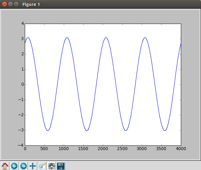
Using practical values for R as 10k, C value can be approximated to 33nF. This oscillator is capable of generating a stable 500 Hz sinusoidal waveform. By changing the resistive and capacitive values of block A and B, we can generate a wide range of frequencies that are supported by the Op Amp because Op Amps have a limited bandwidth it can be functional inside.

It’s worth to note a few facts about generating sine waves using a digital implementation. In analog circuitry, the component values have a tolerance which makes the calculations not perfectly align with the real values. Due to this reason, the actual output will differ from the desired output. In our example to generate 500 Hz sine wave, the capacitors and resistors may have different values and they may have not matched. But with a digital implementation, we can achieve the accuracy and flexibility we require.

External Links:


Continue ReadingSine Wave Generator

Regulating Voltage in PSLab

Electronic components are highly sensitive to voltages and currents across them. Most of the devices in the current market work in the voltage levels of 3.3V, 5V, 12V and 15V. If they are provided with a different voltage than the one required by the vendor, they would not function. If the voltage supplied is higher, they might burn off. The PSLab device requires separate voltage levels such as 3.3V and 5V for its operation.

There are commercial voltage regulators available in the market designed with advanced feedback techniques and models. But we can create out own voltage regulator. In this blog post, I am going to introduce you to a few basic models capable of regulating voltage to a desired level.

Current implementation of PSLab device uses a voltage regulator derived using a zener-resistor combination. This type of regulators have a higher sensitivity to current and their operation may vary when the supplied or the drawn current is lower than the expected values. In order to have a stable voltage regulation, this combination needs to be replaced with a much stable transistor-zener combination.

Before go into much details, let’s get to know a few basic concepts and devices related to.

Zener Diode

Zener DiodeZener diode is a type of diode which has a different operational behavior than the general diode. General diodes allow current to flow only in one direction. If a current in the reverse is applied, they will break and become unusable after a certain voltage level known as Breakdown Voltage. But Zener diodes are specifically designed to function desirably once this break down voltage has been passed and unlike general diode, it can recover back to normal when the voltage is removed or reduced.

Transistor

This is the game changing invention of the 20th century. There are two types of Bipolar Junction Transistors (BJT) available in the market. They are known as NPN and PNP transistors. The difference is based on the polarity of diodes used.

An NPN transistor can be modeled as a combination of two diodes –[NP → PN]– and a PNP transistor can be modeled as –[PN → NP]– using two diodes.

There are three pins to take notice in BJTs. They are illustrated in the diagram shown here;

  1. Base
  2. Collector
  3. Emitter

The amazing fact about BJTs is that the amount of current provided to the Base terminal will control the flow of current going through Collector and Emitter. Also note that always there is a voltage drop across the Base terminal and the Emitter terminal. This typically takes a value of 0.7 V

Voltage Divider

This is the most basic type of voltage regulator. It simply divides the voltage supplied by the battery with the ratio R1:R2. In the following configuration, the output voltage can be calculated using the voltage division rule;

Which is equal to 12 * 100/(100+200) = 4 V

There is a huge drawback with this design. The above calculation is valid only if there is no load impedance is present at the output terminals.

Generally there will be a load impedance and the supplied voltage cannot be easily calculated as the load impedance is unknown to the regulator.

Resistor-Zener Voltage Regulator

Due to the load dependability of the previous model with the load, an improved model can be introduced as follows. This is the current implementation of voltage regulator in PSLab device.

Unlike the previous model, this model ensures that the output voltage will be maintained constant across the output terminals within a range of supply voltage values.

Let’s assume the supply voltage is increased. Then the current flow through the zener diode will increase in order to maintain a constant voltage across the output terminals. In case if the supply voltage drops, then the zener current will decrease and a stable voltage across the output terminals will be maintained.

This design also comes with a slight draw back. This can be explained using the characteristic curve of a zener diode. (Figure is taken from : http://www.electronics-tutorials. ws/diode/diode_7.html)

For a zener diode to maintain a constant voltage level across output terminals, there should be a minimum current flowing through the diode. If this current is not flowing in the zener, there won’t be a regulation. Assume there is a very low load impedance. Then the current supplied by the source will find an easier path to flow other than through the diode. This will affect the regulatory circuit and the desired voltage will not appear across the output terminals.

To compensate the drawback, a much improved design is available using transistors.

Transistor-Zener Voltage Regulator

This is the proposed improvement to the voltage regulatory circuit in PSLab device. In this model, the zener diode is taken away from the load circuit as the current to the load is supplied from the transistor directly. This avoids current limitations to the zener diode had in the previous model and transistor acts as a bridge.

A small current through the Base terminal (1) will support a higher current flow through the output terminal via Collector (2) and Emitter (3). This amplification ratio is in the range of few hundreds for a typical BJT.

A capacitor has been added to compensate ripples from the supply source. If a higher current flow is required through the output terminals, the NPN transistor can be replaced by a Darlington pair.

Using a 5.6 V zener diode and MMBT3904/6 transistors, this model has been implemented in the newest version of PSLab device. They will be supplying a constant voltage of +/- 5V to V+ and V- pins in the device.

External Links:

Continue ReadingRegulating Voltage in PSLab

Constructing and working with Polynomials in the PSLab Android App

PSLab is a device that allows the user to perform a range of science and engineering experiments. PSLab has existing communication library (PSLab Desktop) written in Python. Since we are developing an Android application to operate PSLab, the initial step was to port Python code to JAVA. In PSLab Android application we are using version 3.6.1 of Apache Maths Commons.

NumPy is the package for scientific computing with Python. Polynomials in NumPy can be created using numpy.poly1d. Since some of the files in PSLab Desktop use polynomials, it was important to find a package in JAVA that provides features equivalent to NumPy. Apache Maths Commons fulfilled our needs. It is a Mathematics Library available in JAVA, that provides the means to construct polynomials and perform a range of operations on them. A detailed documentation of the library is available here.

import numpy

p = numpy.poly1d([1, 2, 3])

print(numpy.poly1d(p))

q = p(0.5)

print q

Output:  

1 x2 + 2 x + 3

4.25

Poly1d() function converts a list into polynomials. The first element of the list is the coefficient of the highest degree of the polynomial while the last element is the coefficient of lowest degree of the polynomial. While p(0.5) evaluates polynomial at x = 0.5. 

Now let’s construct polynomials in JAVA using Apache Maths Commons

public class poly {

public static void main(String[] args){

PolynomialFunction p = new PolynomialFunction(new double[]{3, 2, 1});

System.out.println(p);

System.out.println(p.value(0.5));

    }
}

Output:  

3 + 2 x + x^2

4.25

Polynomial Function converts the double array into polynomials. The first element of the array is the coefficient of the lowest degree of the polynomial while the last element is the coefficient of the highest degree of the polynomial. p.value (0.5) evaluates polynomial at x = 0.5.

Other things we can do

  • Find the degree of the polynomial.

Continuing with the above example where polynomial was 3 + 2 x + x^2. p.degree() gives 2 as output which is the degree of the given polynomial.

  • Get the coefficients of the polynomial

p.getCoefficients() returns a double array of the coefficients of the given polynomial. In the above case [3.0, 2.0, 1.0] will be returned.

  • Find derivatives of the polynomial

p.derivative() returns 2 + 2 x which is derivative of polynomial 3 + 2 x + x^2.

  • Add, subtract and multiply two polynomials.

We can add, subtract and multiply 2 polynomials. For example p.multiply(new  Polynomial Function(new double[]{1,2})) returns 3 + 8 x + 5 x^2 + 2 x^3 which is  the product of 3 + 2 x + x^2 and 1 + 2 x

Where are they are used in PSLab?

Polynomials are used in AnalogInputSource.java  to convert raw ADC codes (0=0V , 1023=3.3V ) to voltage values. 

  • calPoly10 = new PolynomialFunction(new double[]{0., 3.3 / 1023, 0.});
  • calPoly12 = new PolynomialFunction(new double[]{0., 3.3 / 4095, 0.});

    Polynomials are also used in DACChannel.java to convert DAC codes to voltage values and vice versa.

  • VToCode = new PolynomialFunction(new double[]{-4095. * intercept / slope, 4095. / slope});                                                    
  • CodeToV = new PolynomialFunction(new double[]{intercept, slope / 4095.});

Continue ReadingConstructing and working with Polynomials in the PSLab Android App

Temporally accurate data acquisition via digital communication pathways in PSLab

This blog post deals with the importance of using a real-time processor for acquiring time dependent data sets. The PSLab already features an oscilloscope, an instrument capable of high speed voltage measurements with accurate timestamps, and it can be used for monitoring various physical parameters such as acceleration and angular velocity as long as there exists a device that can generate a voltage output corresponding to the parameter being measured.  Such devices are called sensors, and a whole variety of these are available commercially.

However, not all sensors provide an analog output that can be input to a regular oscilloscope. Many of the modern sensors use digitally encoded data which has the advantage of data integrity being preserved over long transmission pathways. A commonly used pathway is the I2C data bus, and this blog post will elaborate the challenges faced during continuous data acquisition from a PC, and will explore how a workaround can be managed by moving the complete digital acquisition process to the PSLab hardware in order create a digital equivalent of the analog oscilloscope.

Precise timestamps are essential for extracting waveform parameters such as frequency and phase shifts, which can then be used for calculating physics constants such as the value of acceleration due to gravity, precession, and other resonant phenomena. As mentioned before, oscilloscopes are capable of reliably measuring such data as long as the input signal is an analog voltage, and if a digital signal needs to be recorded, a separate implementation similar to the oscilloscope must be designed for digital communication pathways.

A question for the reader :

Consider a voltmeter capable of making measurements at a maximum rate of one per microsecond.

We would like to set it up to take a thousand readings (n=1000) with a fixed time delay(e.g. 2uS) between each successive sample in order to make it digitize an unknown input waveform. In other words, make ourselves a crude oscilloscope.

Which equipment would you choose to connect this voltmeter to in order to acquire a dataset?

  1. A 3GHz i3 processor powering your favourite operating system, and executing a simple C program that takes n readings in a for loop with a delay_us(2) function call placed inside the loop.
  2. A 10MHz microcontroller , also running a minimal C program that acquires readings in fixed intervals.

To the uninitiated, faster is better, ergo, the GHz range processor trumps the measly microcontroller.

But, we’ve missed a crucial detail here. A regular desktop operating system multitasks between several hundred tasks at a time. Therefore, your little C program might be paused midway in order to respond to a mouse click, or a window resize on any odd chores that the cpu scheduler might feel is more important. The time after which it returns to your program and resumes acquisition is unpredictable, and is most likely of the order of a few milliseconds.

The microcontroller on the other hand, is doing one thing, and one thing only. A delay_us(2) means a 2uS delay with an error margin corresponding to the accuracy of the reference clock used. Simple crystal oscillators usually offer accuracies as good as 30ppm/C, and very low jitter.

Armed with this DIY oscilloscope, we can now proceed to digitize a KHz range since wave or a sound signal from a microphone with good temporal accuracy.

Sample results from the PSLab’s analog oscilloscope

sine wave shown on the oscilloscope
PSLab Oscilloscope showing a 1KHz sinusoidal wave plotted with Matplotlib

If the same were taken via a script that shares CPU time with other processes, the waveform would compress at random intervals due to CPU time unavailability. Starting a new CPU intensive process usually has the effect of the entire waveform appearing compressed because actual time intervals between each sample are greater than the expected time intervals


Implementing the oscilloscope for data buses such as I2C

With regards to the PSLab which already has a reasonably accurate oscilloscope built-in, what happens if one wants to acquire time critical information from sensors connected to the data bus , and not the analog inputs ?

In order acquire such data , the PSLab firmware houses the read routine from I2C in an interrupt function that is invoked at precise intervals by a preconfigured timer’s timeout event. Each sample is stored to an array via a self incrementing pointer.

The I2C address to be accessed, and the bytes to be written before one can start reading data are all pre-configured before the acquisition process starts.

This process then runs at top priority until a preset number of samples have been acquired.Once the host software knows that acquisition should have completed, it fetches the data buffer containing the acquired information.

An example of data being read from a 6-Degree of freedom inertial measurement unit mounted on the pivot of an oscillating physical pendulum.

The plots that overlap accurately with a simulated damped sinusoidal waveform are not possible in the absence of a real-time acquisition system

A 6-DOF sensor connected to the pivot of a physical pendulum.

The sensor in question is the MPU6050 from invensense, used primarily in drones, and other self-stabilising robots.

Its default I2C address is 0x68 ( 104 ) , and 14 registers starting from 0x3B contain data for acceleration along orthogonal axes, temperature, and angular velocity along orthogonal axes. Each of these values is an integer, and is therefore represented by two successive registers. E.g. , 0x3B and 0x3C together make up a 16-bit value for acceleration along the X-axis.


The Final App


Raw Data from a 6-Degree of freedom Inertial Measurement Unit
A least square fit is applied to all 6 datasets (3-axis acceleration, 3-axis angular velocity) from the MPU6050. Extracted parameters show amplitude, frequency, phase and damping coefficient.


Continue ReadingTemporally accurate data acquisition via digital communication pathways in PSLab

Linking Codecov to your Angular2 Project

As a developer, the importance of testing code is well known. Testing source code helps to prevent bugs and syntax errors by cross-checking it with an expected output.
As stated on their official website: “Code coverage provides a visual measurement of what source code is being executed by a test suite”. This information indicates to the software developer where they should write new tests in the effort to achieve higher coverage, and consequently a lower chance of being buggy. Hence nearly every public repository on git uses codecov, a tool to measure the coverage of their source code.

In this blog, we shall see how to link codecov, with a public repository on Github when the code has been written in Angular2(Typescript). We shall assume that the repository uses Travis CI for integration.

STEP 1:
Go to https://codecov.io/gh/ and login to your Github account.

It will now give you the option to chose a repository to add for coverage. Select your repository.

STEP 2:
Navigate to Settings Tab, you should see something like this:

Follow the above-mentioned instructions.

STEP 3:
We now come to one of the most important parts of Codecov integration. Writing the files in our repo to enable this.
We will need three main files:
Travis.yml- which will ensure continuous integration services on your git hosted project
Codecov.yml- to personalise your settings and override the default settings in codecov.”The Codecov Yaml file is the single point of configuration, providing the developers with a transparent and version controlled file to adjust all Codecov settings.” as mentioned in the official website
Package.json- to inform npm of the new dependencies related to codecov, in addition to providing all the metadata to the user.

In .travis.yml, Add the following line:
after_success:

 - bash <(curl -s https://codecov.io/bash)

In codecov.yml, Add the following

Source: https://github.com/codecov/support/wiki/Codecov-Yaml#
 codecov:
 url: "string" # [enterprise] your self-hosted Codecov endpoint
 # ex. https://codecov.company.com
 slug: "owner/repo" # [enterprise] the project's name when using the global upload tokens
 branch: master # the branch to show by default, inherited from your git repository settings
 # ex. master, stable or release
 # default: the default branch in git/mercurial
 bot: username # the username that will consume any oauth requests
 # must have previously logged into Codecov
 ci: # [advanced] a list of custom CI domains
 - "ci.custom.com"
 notify: # [advanced] usage only
 after_n_builds: 5 # how many build to wait for before submitting notifications
 # therefore skipping status checks
 countdown: 50 # number of seconds to wait before checking CI status
 delay: 100 # number of seconds between each CI status check

coverage:
 precision: 2 # how many decimal places to display in the UI: 0 <= value <= 4 round: down # how coverage is rounded: down/up/nearest range: 50...100 # custom range of coverage colors from red -> yellow -> green

notify:
 irc:
 default: # -> see "sections" below
 server: "chat.freenode.net" #*S the domain of the irc server
 branches: null # -> see "branch patterns" below
 threshold: null # -> see "threshold" below
 message: "template string" # [advanced] -> see "customized message" below

gitter:
 default: # -> see "sections" below
 url: "https://webhooks.gitter.im/..." #*S unique Gitter notifications url
 branches: null # -> see "branch patterns" below
 threshold: null # -> see "threshold" below
 message: "template string" # [advanced] -> see "customized message" below

status:
 project: # measuring the overall project coverage
 default: # context, you can create multiple ones with custom titles
 enabled: yes # must be yes|true to enable this status
 target: auto # specify the target coverage for each commit status
 # option: "auto" (must increase from parent commit or pull request base)
 # option: "X%" a static target percentage to hit
 branches: # -> see "branch patterns" below
 threshold: null # allowed to drop X% and still result in a "success" commit status
 if_no_uploads: error # will post commit status of "error" if no coverage reports we uploaded
 # options: success, error, failure
 if_not_found: success # if parent is not found report status as success, error, or failure
 if_ci_failed: error # if ci fails report status as success, error, or failure


patch: # pull requests only: this commit status will measure the
 # entire pull requests Coverage Diff. Checking if the lines
 # adjusted are covered at least X%.
 default:
 enabled: yes # must be yes|true to enable this status
 target: 80% # specify the target "X%" coverage to hit
 branches: null # -> see "branch patterns" below
 threshold: null # allowed to drop X% and still result in a "success" commit status
 if_no_uploads: error # will post commit status of "error" if no coverage reports we uploaded
 # options: success, error, failure
 if_not_found: success
 if_ci_failed: error

changes: # if there are any unexpected changes in coverage
 default:
 enabled: yes # must be yes|true to enable this status
 branches: null # -> see "branch patterns" below
 if_no_uploads: error
 if_not_found: success
 if_ci_failed: error

ignore: # files and folders that will be removed during processing
 - "tests/*"
 - "demo/*.rb"

fixes: # [advanced] in rare cases the report tree is invalid, specify adjustments here
 - "old_path::new_path"

# comment: false # to disable comments
 comment:
 layout: "header, diff, changes, sunburst, suggestions, tree"
 branches: null # -> see "branch patterns" below
 behavior: default # option: "default" posts once then update, posts new if delete
 # option: "once" post once then updates, if deleted do not post new
 # option: "new" delete old, post new
 # option: "spammy" post new

Your package.json should look like this:

{
 "name": "example-typescript",
 "version": "1.0.0",
 "description": "Codecov Example Typescript",
 "main": "index.js",
 "devDependencies": {
 "chai": "^3.5.0",
 "codecov": "^1.0.1",
 "mocha": "^2.5.3",
 "nyc": "^6.4.4",
 "tsd": "^0.6.5",
 "typescript": "^1.8.10"
 },
 "scripts": {
 "postinstall": "tsd install",
 "pretest": "tsc test/*.ts --module commonjs --sourcemap",
 "test": "nyc mocha",
 "posttest": "nyc report --reporter=json && codecov -f coverage/*.json"
 },
 "repository": {
 "type": "git",
 "url": "git+https://github.com/Myname/example-typescript.git"
 },
 /*Optional*/
 "author": "Myname",
 "license": "Lic.name",
 "bugs": {
 "url": "https://github.com/example-typescript-path"
 },
 "homepage": "https://github.com/Myname/example-typescript#readme"
 }

Most of the code in package.json is metadata.
Two major parts of the code above are the devDependencies and the scripts.
In devDependencies, make sure to include the latest versions of all the packages your repository is using.
In scripts:

  • Postinstall – indicates the actions to be performed, once installation is complete.
  • Pretest – is for just before running ng test.
  • Test – indicates what is used while testing.
  • Posttest – is what is run just after testing is complete.

Check this repository for the sample files to generate the reports to be uploaded for Codecov: https://github.com/codecov/example-typescript

Check https://docs.codecov.io/v4.3.6/docs/codecov-yaml for detailed step by step instructions on writing codecov.yaml and https://docs.codecov.io/v4.3.6/docs for any general information

Continue ReadingLinking Codecov to your Angular2 Project

Porting PSLab Libraries – Python to Java

PSLab has existing communication libraries and sensor files in Python which were created during the development of Python Desktop Application.

The initial task and challenge was porting this existing code to Java to be used by the Android App. Since, the python libraries also utilized the object oriented model of programming, porting from Python to Java had the similar code structure and organization.

Common problems faced while porting from Python to Java

  • The most common problem is explicitly assigning data types to variables in Java since Python manages data types on its own. However, most of the time the data types are quite evident from the context of their use and understanding the purpose of the code can make the task much simpler.
  • Another task was migrating the Python data structures to their corresponding Java counterparts like a List in Python represents an ArrayList in Java, similarly a Dictionary corresponds to a HashMap and so on.
  • Some of the sections of the code uses highly efficient libraries like Numpy and Scipy for some mathematical functions. Finding their corresponding Java counterparts in libraries was a challenge. This was partly solved by using Apache Common Math which is a library dedicated for mathematical functions. Some of the functions were directly implemented using this library and for rest of the portions, the code was written after understanding the structure and function of Numpy methods.

While porting the code from Python to Java, some of the steps which we followed:

  • Matching corresponding data-structures

The Dictionary in python…

Gain_scaling = OrderedDict ([('GAIN_TWOTHIRDS', 0.1875), ('GAIN_ONE', 0.125), ('GAIN_TWO', 0.0625), ('GAIN_FOUR', 0.03125), ('GAIN_EIGHT', 0.015625), ('GAIN_SIXTEEN', 0.0078125)])

…was mapped to corresponding Java HashMap in the manner given below. A point to be noted here is for adding elements to a HashMap can be done only from a method and not at the time of declaration of HashMap.

private HashMap <String,Double> gainScaling = new HashMap <String,Double>();

gainScaling.put("GAIN_TWOTHIRDS",0.1875);
gainScaling.put("GAIN_ONE",0.125);
gainScaling.put("GAIN_TWO",0.0625);
gainScaling.put("GAIN_FOUR",0.03125);
gainScaling.put("GAIN_EIGHT",0.015625);
gainScaling.put("GAIN_SIXTEEN",0.0078125);

Similarly, the List in Python can be  be converted to the corresponding ArrayList in Java.

  • Assigning data types and access modifiers to corresponding variables in Java
POWER_ON = 0x01
gain_choices = [RES_500mLx, RES_1000mLx, RES_4000mLx]
ain_literal_choices = ['500mLx', '1000mLx', '4000mLx']
scaling = [2, 1, .25]
private int POWER_ON = 0x01;
public int[] gainChoices = {RES_500mLx,RES_1000mLx,RES_4000mLx};
public String[] gainLiteralChoices = {"500mLx", "1000mLx", "4000mLx"};
public double[] scaling = {2,1,0.25};

Assigning data types and the corresponding access modifiers can get tricky sometimes. So, understanding the code is essential to know whether a variable in limited to the class or needs to be accessed outside the class, whether a variable is int, short, float or double etc.

  • Porting Numpy & Scipy functions to Java using Apache Common Math

For example, this piece of code gives the pitch of acceleration. It uses mathematical functions like arc-tan.

pitchAcc = np.arctan2(accData[1], accData[2]) * 180 / np.pi

The corresponding version of arc-tan in Apache Common Math is used in Java.

double pitchAcc = Math.atan2(accelerometerData[1], accelerometerData[2]) * 180 / pi;
  • Porting by writing the code for Numpy and Scipy functions explicitly

In the code below, rfftfreq is used to calculate the Discrete Fourier Transform(DFT) sample frequencies.

freqs = self.fftpack.rfftfreq(N, d=(xReal[1] - xReal[0]) / (2 * np.pi))

Since, hardly any library in Java supports DFT, the corresponding code for rfftfreq was self-written.

double[] rfftFrequency(int n, double space){
    double[] returnArray = new double[n + 1];
    for(int i = 0; i < n + 1; i++){
        returnArray[i] =  Math.floor(i / 2) / (n * space);
    }
    return Arrays.copyOfRange(returnArray, 1, returnArray.length);
}

After porting of all communication libraries and sensor files are done, the testing of features can also be initiated. Currently, the ongoing development includes porting of the some of the remaining files and working on the the best possible User Interface.

Additional Reading

Continue ReadingPorting PSLab Libraries – Python to Java