Environment Monitoring with PSLab

In this post, we shall explore the working principle and output signals of particulate matter sensors, and explore how the PSLab can be used as a data acquisition device for these.

Working Principle

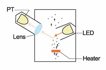
A commonly used technique employed by particulate matter sensors is to study the diffraction of light by dust particles, and estimate the concentration based on a parameter termed the ‘occupancy factor’. The following image illustrates how the most elementary particle sensors work using a photogate, and a small heating element to ensure continuous air flow by convection.

Occupancy Rate

Each time a dust particle of aerodynamic diameters 2.5um passes through the lit area, a phenomenon called Mie scattering which defines scattering of an electromagnetic plane wave by a homogenous sphere of diameter comparable to the wavelength of incident light, results in a photo-signal to be detected by the photosensor.  In more accurate dust sensors, a single wavelength source with a high quality factor such as a laser is used instead of LEDs which typically have broader spectra.

The signal output from the photosensor is in the form of intermittent digital pulses whenever a particle is detected. The occupancy ratio can be determined by measuring the sum total of time when a positive signal was output from the sensor to the total averaging time. The readings can be taken over a fairly long amount of time such as 30 seconds in order to get a more accurate representation of the occupancy ratio.

Using the Logic analyzer to capture and interpret signals

The PSLab has a built-in logic analyzer that can acquire data signals up to 67 seconds long at its highest sampling rate, and this period is more than sufficient to record and interpret a dataset from a dust sensor. An inexpensive dust sensor, DSM501A was chosen for the readings, and the following results were obtained

Dust sensor readings from an indoor, climate controlled environment. After the 100 second mark, the windows were opened to expose the sensor to the outdoor environment.

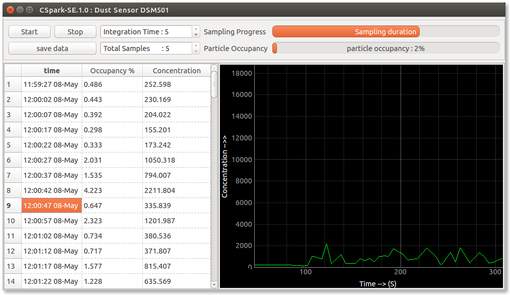
A short averaging time has resulted in large fluctuations in the readings, and therefore it is important to maintain longer averaging times for stable measurements.

Recording data with a python script instead of the app

The output of the dust sensor must be connected to ID1 of the PSLab, and both devices must share a common ground which is a prerequisite for exchange of DC signals. All that is required is to start the logic analyzer in single channel mode, wait for a specified averging time, and interpret the acquired data

Record_dust_sensor.py

from PSL import sciencelab   #import the required library
import time
import numpy as np
I = sciencelab.connect()           #Create the instance
I.start_one_channel_LA(channel='ID1',channel_mode=1,trigger_mode=0)  #record all level changes
time.sleep(30)   #Wait for 30 seconds while the PSLab gathers data from the dust sensor
a,_,_,_,e =I.get_LA_initial_states()      #read the status of the logic analyzer
raw_data =I.fetch_long_data_from_LA(a,1)  #fetch number of samples available in chan #1
I.dchans[0].load_data(e,raw_data)  
stamps =I.dchans[0].timestamps    #Obtain a copy of the timestamps
if len(stamps)>2:   #If more than two timestamps are available (At least one dust particle was detected
		if not self.I.dchans[0].initial_state:   #Ensure the starting position of timestamps
			stamps = stamps[1:] - stamps[0]   # is in the LOW state
	diff = np.diff(stamps)   #create an array of individual time gaps between successive level changes


	lows = diff[::2]      #Array of time durations when a particle was not present
	highs = diff[1::2]    #Array of time durations when a particle was present
	low_occupancy = 100*sum(lows)/stamps[-1] #Occupancy ratio
print (low_occupancy) # datasheets of individual dust sensors also provide a mathematical
                      #equation to interpret the occupancy ratio as concentration of
				#particulate matter

Further Reading, and application notes:

[1] LED based  dust Sensor application note

Continue ReadingEnvironment Monitoring with PSLab

Analyzing Sensor Data on PSLab

PSLab Android App and Desktop app have the functionality of reading data from the sensors. The raw sensor data received is in the form of a long string and needs to parsed to understand what the data actually conveys.

The sensor data is unique in terms of volume of data sent, the units of measurement of the data etc., however none of this is reflected in the raw data. The blog describes how the sensor data received by the Android/Desktop app is parsed, interpreted and finally presented to the user for viewing.

The image below displays the raw data sent by the sensors

blog_post_9_2

Fig: Raw Sensor data displayed below the Get Raw button

  • In order to understand the data sent from the sensor, we need to understand what the sensor does.
    • For example, HMC5883L is a 3-axis magnetometer and it returns the value of the magnetic field in the x, y & z axes in the order of nanoTeslas.
    • Similarly, the DAC of PSLab – MCP4728 can also be used like other sensors, it returns the values of channels in millivolts.
    • The sensor MPU6050 being 3-axes accelerometer & gyroscope which returns the values of acceleration & angular momentum of the x, y & z axes in their SI units respectively.
  • Each sensor has a sensitivity value. The sensitivity of the sensor can be modified to adjust the accuracy of the data received. For PSLab, the data returned is a float number with each data point having 4 bytes of memory with the highest sensitivity. Although sensitivity is not a reliable indicator of the accuracy of the data. Each value received has a lot of trailing values after the decimal and it is evident that no sensor can possibly achieve accuracy that high, so the data after 2-3 decimal places is garbage and not taken into consideration.
  • Some sensors are configurable up to a great extent like MPU6050 where limits can also be set on the range of data, volume of data sent etc. whereas some are not configurable and are just meant for sending the data at regular intervals.
  • In order to parse the above data, if the sensor returns a single value, then the data is ready to be used. However, in most cases like above where the sensors return multiple values, the data stream can be divided into equal parts since each value occupies equal space and each value can be stored in different variables.
  • The stored data has to be presented to the user in a better understandable format where it is clear that what each value represents. For example, in case of the 3 axes sensors, the data of each axis must be distinctly represented to the user.

Shown below are the mock-ups of the sensor UIs in which each value has been distinctly represented.


Fig: Mock-ups for the sensor UIs (a) – HMC5883L (b) – MPU6050

Each UI has a card to display those values. These values are updated in real time and there are additional options to plot the data received in real time and in some cases also configure the sensor. In addition to that there are features for data logging where the data is recorded for a given time interval specified by the user and on completion of recording, calculations like the mean, standard deviation etc. are presented to the user.

Additional Resources

  1. Analyzing sensor data using Arduino, similar to method for PSLab – http://tronixstuff.com/2014/01/21/online-data-analysis-arduino-plotly/
  2. YouTube video to understand analysis of data from MPU6050 in Arduino – https://www.youtube.com/watch?v=taZHl4Mr-Pk

Continue ReadingAnalyzing Sensor Data on PSLab

Creating Multiple Device Compatible Layouts in PSLab Android

The developer’s goal is that PSLab Android App as an app should run smoothly on all the variety of Android devices out in the market. There are two aspects of it – the app should be able to support maximum number of Android versions possible which is related to the core software part and the other being the app should be able to generate the same user experience on all sizes of screens. This post focuses on the later.

There are a whole range of android devices available in the market right from 4 inch mobile phones to 12 inch tablets and the range in the screen sizes is quite large. So, the challenge in front of app designers is to make the app compatible with the maximum  number of devices without doing any specific tweaks related to a particular resolution range. Android has its mechanism of scaling the app as per the screen size and it does a good job almost all the time, however, still there are cases where android fails to scale up or scale down the app leading to distorted layout of the app.

This blog discusses some of the tricks that needs to be kept in mind while designing layouts that work independent of screen sizes.

Avoid using absolute dimensions

It is one of the most common things to keep in mind before starting any UI design. Use of absolute dimensions like px, inch etc. must be avoided every time as they are fixed in size and don’t scale up or scale down while screen sizes are changed. Instead relative dimensions like dp should be used which depend on the resolution and scale up or scale down. ( It’s a fair assumption that bigger screens will have better resolution compared to the smaller ones although exceptions do exist) .

Ensure the use of correct layout/View group

Since, android provides a variety of layouts like Linearlayout, Constrainedlayout, Relativelayout, Tablelayout and view groups like ScrollView, RecyclerView, ListView etc. it is often confusing to know which layout/viewgroup should be used. The following list gives a rough idea of when to use a particular layout or view group.

  • Linearlayout – Mostly used for simple designs when the elements are stacked in ordered horizontal/vertical fashion and it needs explicit declaration of orientation.
  • Relativelayout – Mostly used when the elements need to defined relative to the parent or the neighbouring elements. Since, the elements are relative, there is no need to define the orientation.
  • Constraintlayout – It has all the features of Relativelayout and in addition a feature of adding constraints to the child elements or neighbouring elements.
  • Tablelayout – Tablelayout is helpful to when all the views/widgets are arranged in an ordered fashion.

All the above layouts can be used interchangeably most of the times, however, certain cases make some more favourable than others like when than views/ widgets are not present in an organised manner, it is better to stick to Linearlayout or Relativelayout.

  • ListView – Used when the views/ widgets in a screen are repeated, so using a listview ensures that the volume of the code is reduced and all the repetitive views are identical in nature.
  • RecyclerView – More of an improved version of ListView. It is recommended to use this view over ListView. Additionally this view group supports features like swipe to refresh.
  • ScrollView – Used when the UI screen cannot fit within the given screen space. ScrollView supports one direct child layout. So, to implement a scrollview, all the views must be under a particular layout and then masked by scrollview.

Choosing the correct layout or view group would help to create a better UI.

Use of layout_weight

Ensuring the layout width assigned in XML file covers the entire width on the screen. For ensuring this, one possible solution is to use layout_weight instead of layout_width.

Example –

<TextView
   android:id="@+id/tv_control_read9"
   android:layout_width="0dp"
   android:layout_weight="1"
   android:layout_height="30dp"
   android:layout_marginTop="10dp"
/>


In order to use layout_weight, layout_width must be set to 0 else it would interfere with the width and as layout_width is a compulsory parameter it cannot be omitted. Layout weight can be any number and the space is allocated to each view in proportion to the weights assigned. Since it does not involve numerical dimensions, the distribution would be uniform for all types of screens. The result is clearly evident here. The same UI in different screen sizes is displayed below.

blog_post_8_2

Fig: Screenshot taken on a 6” phone and on a 4” phone. Although the screen area of 4” phone is 44% that of the 6” phone, the UIs are identically the same.

Create different layout directories for different resolutions

  • Creating different layouts for different screen sizes ensures that the limitations of smaller screen sizes are taken care of and the advantages offered by bigger screen sizes are put to the best use.
  • The Android documentation here mentions the conventions to be followed while designing.
  • Although over the years, android has become better at auto-adjusting layouts for different screen sizes. However, if the no. of views and widgets are high, auto-adjusting does not work well as in case of PSLab and it is better to create different sets of layouts.
  • As evident from the picture of the 8” tablet, although the auto-adjusted layout is manageable, the layout looks stretched and does not utilize the entire screen space, so it a better UI can be made by creating a dedicated layout directory for bigger screens.

Additional resources


Continue ReadingCreating Multiple Device Compatible Layouts in PSLab Android

Using Sensors with PSLab Android App

The PSLab Android App as of now supports quite a few sensors. Sensors are an essential part of many science experiments and therefore PSLab has a feature to support plug & play sensors. The list of sensors supported by PSLab can be found here.

  • AD7718 – 24-bit 10-channel Low voltage Low power Sigma Delta ADC
  • AD9833 – Low Power Programmable Waveform generator
  • ADS1115 – Low Power 16 bit ADC
  • BH1750 – Light Intensity sensor
  • BMP180 – Digital Pressure Sensor
  • HMC5883L – 3-axis digital magnetometer
  • MF522 – RFID Reader
  • MLX90614 – Infrared thermometer
  • MPU6050 – Accelerometer & gyroscope
  • MPU925x – Accelerometer & gyroscope
  • SHT21 – Humidity sensor
  • SSD1306 – Control for LED matrix
  • Sx1276 – Low Power Long range Transceiver
  • TSL2561 – Digital Luminosity Sensor

All the sensors except Sx1276 communicate using the I2C protocol whereas the Sx1276 uses the SPI protocol for communication. There is a dedicated set of ports on the PSLab board for the communication under the label I2C with the ports named 3.3V, GND, SCL & SDA.

blog_post_7_1

Fig; PSLab board sketch

Any I2C sensor has ports named 3.3V/VCC, GND, SCL, SDA at least along with some other ports in some sensors. The connections are as follows:

  1. 3.3V on PSLab – 3.3V/VCC on sensor
  2. GND on PSLab – GND on sensor
  3. SCL on PSLab – SCL on sensor
  4. SDA on PSLab – SDA on sensor

The diagram here shows the connections

For using the sensors with the Android App, there is a dedicated I2C library written in communication in Java for the communication. Each sensor has its own specific set of functionalities and therefore has its own library file. However, all these sensors share some common features like each one of them has a getRaw method which fetches the raw sensor data. For getting the data from a sensor, the sensor is initially connected to the PSLab board.

The following piece of code is responsible for detecting any devices that are connected to the PSLab board through the I2C bus. Each sensor has it’s own unique address and can be identified using it. So, the AutoScan function returns the addresses of all the connected sensors and the sensors can be uniquely identified using those addresses.

public ArrayList<Integer> scan(Integer frequency) throws IOException {
	if (frequency == null) frequency = 100000;
	config(frequency);
	ArrayList<Integer> addresses = new ArrayList<>();
	for (int i = 0; i < 128; i++) {
		int x = start(i, 0);
		if ((x & 1) == 0) {
			addresses.add(i);
		}
		stop();
	}
	return addresses;
}


As per the addresses fetched, the sensor library corresponding to that particular sensor can be imported and the getRaw method can be called. The getRaw method will return the raw sensor data. For example here is the getRaw method of ADS1115.

public int[] getRaw() throws IOException, InterruptedException {
	String chan = typeSelection.get(channel);
	if (channel.contains("UNI"))
		return new int[]{(int) readADCSingleEnded(Integer.parseInt(chan))};
	else if (channel.contains("DIF"))
		return new int[]{readADCDifferential(chan)};
	return new int[0];
}

Here the raw data is returned in the form of voltages in mV.

Similarly, the other sensors return some values like luminosity sensor TSL2561 returns values of luminosity in Lux, the accelerometer & gyroscope MPU6050 returns the angles of the 3-axes.

In order to initiate the process of getting raw data from the sensor in Sensor Activity, the object for the sensor is created and the method of getRaw is called. The following is the implementation for ADS1115. The rest of the sensors also have an implementation similar to this. There are try-catch statements in the code to handle some of the exceptions thrown during process of method calls.

ADS1115 ADS1115 = null;
try {
	ADS1115 = new ADS1115(i2c);
} catch (IOException | InterruptedException e) {
	e.printStackTrace();
}

int[] dataADS1115 = null;
String datadispADS1115 = null;
try {
	if (ADS1115 != null) {
		dataADS1115 = ADS1115.getRaw();
	}
} catch (IOException | InterruptedException e) {
	e.printStackTrace();
}

if (dataADS1115 != null) {
	for(int i = 0; i < dataADS1115.length; i++)
		datadispADS1115 += String.valueOf(dataADS1115[i]);
	}

tvSensorGetRaw.setText(datadispADS1115);


Additional Resources

  1. Sensor implementation in PSLab Python repository – https://github.com/fossasia/pslab-python/tree/development/PSL/SENSORS
  2. Using the sensors with Arduino in case you have worked with Arduino before – The basic connections are same as PSLab http://www.instructables.com/id/Arduino-MPU-6050-Getting-It-to-Work/

Continue ReadingUsing Sensors with PSLab Android App

Creating Custom Components in the PSLab Android App

PSLab Android App supports a lot of features and each of these features need components & views for their implementation. A typical UI of PSLab is shown in the figure below. Considering the number of views & components used in the figure, implementation of each view & component separately would lead to a huge volume of repetitive and inefficient code. As it is evident that the EditText and two buttons beside it keep repeating a lot, it is wiser to create a single custom component consisting of an EditText and two buttons. This not only leads to efficient code but also results in a drastic reduction of the volume of code.

Android has a feature which allows creating components. For almost all the cases, the pre-defined views in Android serve our purpose of creating the UIs. However, sometimes there is a need to create custom components to reduce code volume and improve quality. Custom components are used when a particular set of component needed by us is not present in the Android view collection or when a pattern of components is frequently repeated or when we need to reduce the code complexity.

The above set can be replaced by defining a custom component which includes an edittext and two buttons and then treating it like just any other component. To get started with creating a custom component, the steps are the following:

Create a layout for the custom component to be designed

<?xml version="1.0" encoding="utf-8"?>
<LinearLayout xmlns:android="http://schemas.android.com/apk/res/android"
   android:orientation="horizontal" android:layout_width="match_parent"
   android:layout_height="match_parent">

   <Button
       android:id="@+id/button_control_plus"
       android:layout_width="0dp"
       android:layout_weight="0.5"
       android:layout_height="20dp"
       android:background="@drawable/button_minus" />

   <EditText
       android:id="@+id/edittext_control"
       android:layout_width="0dp"
       android:layout_weight="2"
       android:layout_height="24dp"
       android:layout_marginTop="@dimen/control_margin_small"
       android:inputType="numberDecimal"
       android:padding="@dimen/control_edittext_padding"
       android:background="@drawable/control_edittext" />

   <Button
       android:id="@+id/button_control_minus"
       android:layout_width="0dp"
       android:layout_weight="0.5"
       android:layout_height="20dp"
       android:background="@drawable/button_plus" />
</LinearLayout>

The layout file edittext_control.xml is created with three views and each one of them has been assigned an ID along with all the other relevant parameters.

Incorporate the newly created custom layout in the Activity/Fragment layout file

<org.fossasia.pslab.others.Edittextwidget
       android:id="@+id/etwidget_control_advanced1"
       android:layout_height="wrap_content"
       android:layout_width="0dp"
       android:layout_weight="2"
       android:layout_marginLeft="@dimen/control_margin_small"
       android:layout_marginStart="@dimen/control_margin_small"
/>

The custom layout can be added the activity/fragment layout just like any other view and can be assigned properties similarly.

Create the activity file for the custom layout

public class Edittextwidget extends LinearLayout{

   private EditText editText;
   private Button button1;
   private Button button2;
   private double leastCount;
   private double maxima;
   private double minima;

 
   public Edittextwidget(Context context, AttributeSet attrs, int defStyle) {
       super(context, attrs, defStyle);
       applyAttrs(attrs);
   }

   public Edittextwidget(Context context, AttributeSet attrs) {
       super(context, attrs);
       applyAttrs(attrs);
   }

   public Edittextwidget(Context context) {
       super(context);
   }

  public void init(Context context, final double leastCount, final double minima, final double maxima) {
       View.inflate(context, R.layout.edittext_control, this);
       editText = (EditText) findViewById(R.id.edittext_control);
       button1 = (Button) findViewById(R.id.button_control_plus);
       button2 = (Button) findViewById(R.id.button_control_minus);

       button1.setOnClickListener(new OnClickListener() {
           @Override
           public void onClick(View v) {
               Double data = Double.valueOf(editText.getText().toString());
               data = data - leastCount;
               data = data > maxima ? maxima : data;
               data = data < minima ? minima : data;
               editText.setText(String.valueOf(data));
           }
       });

       button2.setOnClickListener(new OnClickListener() {
           @Override
           public void onClick(View v) {
               Double data = Double.valueOf(editText.getText().toString());
               data = data + leastCount;
               data = data > maxima ? maxima : data;
               data = data < minima ? minima : data;
               editText.setText(String.valueOf(data));
           }
       });
   }

   private void applyAttrs(AttributeSet attrs) {
       TypedArray a = getContext().obtainStyledAttributes(attrs, R.styleable.Edittextwidget);
       final int N = a.getIndexCount();
       for (int i = 0; i < N; ++i) {
           int attr = a.getIndex(i);
           switch (attr) {
               case R.styleable.Edittextwidget_leastcount:
                   this.leastCount = a.getFloat(attr, 1.0f);
                   break;
               case R.styleable.Edittextwidget_maxima:
                   this.maxima = a.getFloat(attr, 1.0f);
                   break;
               case R.styleable.Edittextwidget_minima:
                   this.minima = a.getFloat(attr, 1.0f);
           }
       }
       a.recycle();
   }
}

In the activity file Editextwidget.java, the views of the custom layout are defined and functionalities are assigned to them. For example, here there are two buttons which work as increment/decrement buttons and an edittext which takes numeric input. The buttons are initiated just like the way they are done in other activity/fragment using OnClickListener.

Define the attributes for the custom layout

<declare-styleable name="Edittextwidget">
     <attr name="leastcount" format="float" />
     <attr name="maxima" format="float" />
     <attr name="minima" format="float" />
</declare-styleable>

The attributes for the custom layout are defined in the attrs.xml file. Each attribute is assigned a name and a format which can be int, float, double, string etc.

Finally call the methods of the custom layout from the desired activity/fragment

Edittextwidget etwidgetControlAdvanced1 = (Edittextwidget)view.findViewById(R.id.etwidget_control_advanced1);

etwidgetControlAdvanced1.init(getContext(), 1.0, 10.0, 5000.0);

The init method of Edittextwidget.java is called while passing the relevant parameters like context, least count, maxima and minima.

Additional Resources on Custom Components

  1. Official Android Guide on Custom components – https://developer.android.com/guide/topics/ui/custom-components.html
  2. Simple example of creating a custom component to get started – https://www.tutorialspoint.com/android/android_custom_components.htm
Continue ReadingCreating Custom Components in the PSLab Android App

Trigger Controls in Oscilloscope in PSLab

PSLab Desktop App has a feature of oscilloscope. Modern day oscilloscopes found in laboratories support a lot of advanced features and addition of trigger controls in oscilloscope was one such attempt in adding an advanced feature in the oscilloscope. As the current implementation of trigger is not robust enough, this feature would help in better stabilisation of waveforms.

Captured waveforms often face the problem of distortion and trigger helps to solve this problem. Trigger in oscilloscope is an essential feature for signal characterisation.  as it synchronises the horizontal sweep of the oscilloscope to the proper point of the signal. The trigger control enables users to stabilise repetitive waveforms as well as capture single-shot waveforms. By repeatedly displaying similar portion of the input signal, the trigger makes repetitive waveform look static. In order to visualise how an oscilloscope looks with or without a trigger see the following figures below.

blog_post_5_1

blog_post_5_2

Fig 1: (a) Without trigger  (b) With trigger

The Fig:1(a) is the actual waveform received by the oscilloscope and it can be easily noticed that interpreting it is confusing due to the overlapping of multiple waveforms together. So, in Fig:1(b) the trigger control stabilises the waveforms and captures just one waveform.

In general the commonly used trigger modes in laboratory oscilloscopes are:-

  • Auto – This trigger mode allows the oscilloscope to acquire a waveform even when it does not detect a trigger condition. If no trigger condition occurs while the oscilloscope waits for a specific period (as determined by the time-base setting), it will force itself to trigger.
  • Normal – The Normal mode allows the oscilloscope to acquire a waveform only when it is triggered. If no trigger occurs, the oscilloscope will not acquire a new waveform, and the previous waveform, if any, will remain on the display.
  • Single – The Single mode allows the oscilloscope to acquire one waveform each time you press the RUN button, and the trigger condition is detected.
  • Scan – The Scan mode continuously sweeps waveform from left to right.

Implementing Trigger function in PSLab

PSLab has a built in basic functionality of trigger control in the configure_trigger method in sciencelab.py. The method gets called when trigger is enabled in the GUI. The trigger is activated when the incoming wave reaches a certain voltage threshold and the PSLab also provides an option of either selecting the rising or falling edge for trigger. Trigger is especially useful in experiments handling waves like sine waves, square wave etc. where trigger helps to get a clear picture.

In order to initiate trigger in the PSLab desktop app, the configure_trigger method in sciencelab.py is called. The configure_trigger method takes some parameters for input but they are optional. If values are not specified the default values are assumed.

def configure_trigger(self, chan, name, voltage, resolution=10, **kwargs):
        
  prescaler = kwargs.get('prescaler', 0)
        try:
            self.H.__sendByte__(CP.ADC)
            self.H.__sendByte__(CP.CONFIGURE_TRIGGER)
            self.H.__sendByte__(
                (prescaler << 4) | (1 << chan))  
            if resolution == 12:
                level = self.analogInputSources[name].voltToCode12(voltage)
                level = np.clip(level, 0, 4095)
            else:
                level = self.analogInputSources[name].voltToCode10(voltage)
                level = np.clip(level, 0, 1023)

            if level > (2 ** resolution - 1):
                level = (2 ** resolution - 1)
            elif level < 0:
                level = 0

            self.H.__sendInt__(int(level))  # Trigger
            self.H.__get_ack__()
        
        except Exception as ex:
  	    self.raiseException(ex, "Communication Error , Function : " + inspect.currentframe().f_code.co_name)

The method takes the following parameters in the method call

  • chan – Channel . 0, 1,2,3. corresponding to the channels being recorded by the capture routine(not the analog inputs).
  • name – The name of the channel. ‘CH1’… ‘V+’.
  • voltage – The voltage level that should trigger the capture sequence(in Volts).

The similar feature will also be used in oscilloscope in the Android app with the code corresponding to this method  in ScienceLab written in Java.

Additional Resources

  1. Read more about Trigger here – http://www.radio-electronics.com/info/t_and_m/oscilloscope/oscilloscope-trigger.php
  2. Learn more about trigger modes in oscilloscopes – https://www.picotech.com/library/oscilloscopes/advanced-digital-triggers
  3. PSLab Python repository to know the underlying code – https://github.com/fossasia/pslab-python


Continue ReadingTrigger Controls in Oscilloscope in PSLab

How to Collaborate Design on Hardware Schematics in PSLab Project

Generally ECAD tools are not built to support collaborative features such as git in software programming. PSLab hardware is developed using an open source ECAD tool called KiCAD. It is a practice in the electronic industry to use hierarchical blocks to support collaboration. One person can work on a specific block having rest of the design untouched. This will support a workaround to have a team working on a one hardware design just like a software design. In PSLab hardware repository, many developers can work simultaneously using this technique without having any conflicts in project files.

Printed Circuit Board (PCB) designing is an art. The way the components are placed and how they are interconnected through different type of wires and pads, it is an art for hardware designing engineers. If they do not use auto-route, PCB design for the same schematic will be quite different from one another.

There are two major approaches in designing PCBs.

  • Top Down method
  • Bottom Up method

Any of these methods can be implemented in PSLab hardware repository to support collaboration by multiple developers at the same time.

Top Down Method

In this method the design is starting from the most abstract definitions. We can think of this as a black box with several wires coming out of it. The user is aware of how to use the wires and to which devices they need to be connected. But the inside of the black box is not visible. Then a designer can open up this box and break the design down to several small black boxes which can perform a subset of functionalities the bigger black box did. He can go on breaking it down to even smaller boxes and reach the very bottom where basic components are found such as transistors, resistors, diodes etc.

Bottom Up Method

In the bottom up method, the opposite approach of the top down method is used. Small parts are combined together to design a much bigger part and they are combined together to build up an even bigger part which will eventually create the final design. Our human body is a great example for a use of bottom up method. Cells create organ; organs create systems and systems create the body.

Designing Top Down Designs using KiCAD

In PCB designing, the designers are free to choose whatever the approach they prefer more suitable for their project. In this blog, the Top Down method is used to demonstrate how to create a design from the abstract concepts. This will illustrate how to create a design with one layer deep in design using hierarchical blocks. However, these design procedures can be carried out as many times as the designer want to create depending on the complexity of the project.

Step 01 – Create a new project in KiCAD

Step 02 – Open up Eeschema to begin the design

Step 03 – Create a Hierarchical Sheet

Step 04 – Place the hierarchical sheet on the design sheet and give it a name

Step 05 – Enter sheet

Step 06 – Place components and create a schematic design inside the sheet and place hierarchical labels

Step 07 – Define the labels as input or output and give them an identifier. Once done, place them on appropriate places and connect with wires

Step 08 – Go back to main sheet to complete the hierarchical block

Step 09 – Place hierarchical pins on the block

Click on the “Place hierarchical pin” icon from the toolbar and click on the block. The pins can be placed on anywhere on the block. As a convention, input pins are placed on the left side and the output pins are placed on the right side of the block.

Step 10 – Complete the circuit

Resources:

Continue ReadingHow to Collaborate Design on Hardware Schematics in PSLab Project

Generate Sine Waves with PSLab Device

Sine wave is type of a waveform with much of a use in frequency related studies in laboratories as well as power electronics to control the level of input to devices. PSLab device  is capable of generating sine waves with a very high accuracy using PSLab-firmware and a set of filters implemented in the PSLab-hardware.

How Sine Wave is generated in PSLab Device

PSLab device uses a PIC micro-controller as its main processor. It has several pins which can generate square pulses at different duty cycles. These are known as PWM pins. PWM waves are a type of a waveform with the shape resembling a set of square pulses. They have an attributed called ‘Duty Cycle’ which varies between 0% to 100%. A PWM wave with 0% duty cycle means simply a zero amplitude block of square pulses repeating at every period. When duty cycle is set to 100%, it is a set of square pulses with the highest amplitude throughout the period repeating in every period. The following figure illustrates how the PWM wave changes according to its duty cycle. Image is extracted from http://static.righto.com/images/pwm1.gif PSLab device is capable of generating this type of pulses with arbitrary duty cycles as per user requirements.

In this context where sine waves are generated, these PWM pins are used to generate a Sinusoidal Pulse Width Modulated (SPWM) waveform as the first step to output a sine wave with high frequency accuracy. The name SPWM is derived from the fact that the duty cycle of the waveform follows an alternatively increasing and decreasing pattern as illustrated in the figure below.

Deriving a set of duty cycles which follows a sinusoidal pattern is a redundant task. Without deriving them mathematically, PSLab firmware has four hard-coded sine_tables which stores different duty cycle values related to a SPWM waveform. These sine_tables in the firmware related to different resolutions set by the PSLab device user. The following code block is extracted from PSLab firmware related to one of the sine_tables. It is used to generate the SPWM wave with 512 data points. Each data point represents a square pulse with a different pulse width. The duty ratio is calculated from dividing an entry by the value 512 and converting it to a percentage.

sineTable1[] = {256, 252, 249, 246, 243, 240, 237, 234, 230, 227, 224, 221, 218, 215, 212, 209, 206, 203, 200, 196, 193, 190, 187, 184, 181, 178, 175, 172, 169, 166, 164, 161, 158, 155, 152, 149, 146, 143, 141, 138, 135, 132, 130, 127, 124, 121, 119, 116, 114, 111, 108, 106, 103, 101, 98, 96, 93, 91, 89, 86, 84, 82, 79, 77, 75, 73, 70, 68, 66, 64, 62, 60, 58, 56, 54, 52, 50, 48, 47, 45, 43, 41, 40, 38, 36, 35, 33, 32, 30, 29, 27, 26, 25, 23, 22, 21, 19, 18, 17, 16, 15, 14, 13, 12, 11, 10, 9, 8, 8, 7, 6, 6, 5, 4, 4, 3, 3, 2, 2, 2, 1, 1, 1, 0, 0, 0, 0, 0, 0, 0, 0, 0, 0, 0, 1, 1, 1, 2, 2, 2, 3, 3, 4, 4, 5, 6, 6, 7, 8, 8, 9, 10, 11, 12, 13, 14, 15, 16, 17, 18, 19, 21, 22, 23, 25, 26, 27, 29, 30, 32, 33, 35, 36, 38, 40, 41, 43, 45, 47, 48, 50, 52, 54, 56, 58, 60, 62, 64, 66, 68, 70, 73, 75, 77, 79, 82, 84, 86, 89, 91, 93, 96, 98, 101, 103, 106, 108, 111, 114, 116, 119, 121, 124, 127, 130, 132, 135, 138, 141, 143, 146, 149, 152, 155, 158, 161, 164, 166, 169, 172, 175, 178, 181, 184, 187, 190, 193, 196, 200, 203, 206, 209, 212, 215, 218, 221, 224, 227, 230, 234, 237, 240, 243, 246, 249, 252, 256, 259, 262, 265, 268, 271, 274, 277, 281, 284, 287, 290, 293, 296, 299, 302, 305, 308, 311, 315, 318, 321, 324, 327, 330, 333, 336, 339, 342, 345, 347, 350, 353, 356, 359, 362, 365, 368, 370, 373, 376, 379, 381, 384, 387, 390, 392, 395, 397, 400, 403, 405, 408, 410, 413, 415, 418, 420, 422, 425, 427, 429, 432, 434, 436, 438, 441, 443, 445, 447, 449, 451, 453, 455, 457, 459, 461, 463, 464, 466, 468, 470, 471, 473, 475, 476, 478, 479, 481, 482, 484, 485, 486, 488, 489, 490, 492, 493, 494, 495, 496, 497, 498, 499, 500, 501, 502, 503, 503, 504, 505, 505, 506, 507, 507, 508, 508, 509, 509, 509, 510, 510, 510, 511, 511, 511, 511, 511, 511, 511, 511, 511, 511, 511, 510, 510, 510, 509, 509, 509, 508, 508, 507, 507, 506, 505, 505, 504, 503, 503, 502, 501, 500, 499, 498, 497, 496, 495, 494, 493, 492, 490, 489, 488, 486, 485, 484, 482, 481, 479, 478, 476, 475, 473, 471, 470, 468, 466, 464, 463, 461, 459, 457, 455, 453, 451, 449, 447, 445, 443, 441, 438, 436, 434, 432, 429, 427, 425, 422, 420, 418, 415, 413, 410, 408, 405, 403, 400, 397, 395, 392, 390, 387, 384, 381, 379, 376, 373, 370, 368, 365, 362, 359, 356, 353, 350, 347, 345, 342, 339, 336, 333, 330, 327, 324, 321, 318, 315, 311, 308, 305, 302, 299, 296, 293, 290, 287, 284, 281, 277, 274, 271, 268, 265, 262, 259};


The frequency of the sine wave is achieved using interrupts generated at different time intervals depending on the frequency set by the user. The accuracy of the frequency depends on the number of elements in the sine table array which is known as resolution. As the number of points in the table increases, the accuracy will be increased or resolution will be high. PSLab uses Timer3 and Timer4 counters available in the PIC micro-controller to generate the interrupt time intervals. If the required frequency is f, the interrupt time interval can be derived as

Interrupt time = f/512

The derived SPWM waveform will be then passed through a cascaded setup of Op Amp and RC filter as in Figure 1 to cut off the high frequency components and combine the square pulses in such a manner that a smoother waveform is derived resembling a sine wave.

Filter Circuit in PSLab

Figure 1

This is an inverting filter circuit designed using Op Amps available in PSLab-hardware. The SPWM waveform will be connected to the circuit through R1 resistor. It uses C1 capacitor which creates a short circuit path to high frequency components to ground which will let only the low frequency components to pass through. This will smoothen the square waves reducing the sharp edges forming a simple RC filter circuit.

The C2 capacitor plays an important role in generating the sine wave. It will compensate any voltage drops and absorb excess voltage levels that might occur during transition to let the output waveform follow a path which is similar to a smooth sine wave.

The output waveform can be observed from the SINE1 pin of the PSLab device. As in this schematic, it is the ‘Sine Wave’ pin to the right starting from the Op Amp output.

Resources:

Continue ReadingGenerate Sine Waves with PSLab Device

Curve-Fitting in the PSLab Android App

One of the key features of PSLab is the Oscilloscope. An oscilloscope allows observation of temporal variations in electrical signals. Its main purpose is to record the input voltage level at highly precise intervals and display the acquired data as a plot. This conveys information about the signal such as the amplitude of fluctuations, periodicity, and the level of noise in the signal. The Oscilloscope helps us to observe varying the waveform of electronic signals, it is obvious it measures a series of data points that need to be plotted on the graph of the instantaneous signal voltage as a function of time.

When periodic signals such as sine waves or square waves are read by the Oscilloscope, curve fitting functions are used to construct a curve that has the best fit to a series of data points. Curve fitting is also used on data points generated by sensors, for example, a damped sine fit is used to study the damping of the simple pendulums. The curve fitting functions are already written in Python using libraries like numpy and scipy. analyticsClass.py provides almost all the curve fitting functions used in PSLab. For the Android, implementation we need to provide the same functionality in Java.

More about Curve-fitting

Technically speaking, Curve-fitting is the process of constructing a curve or mathematical function, that has the best fit to a series of data points, possibly subject to constraints.

Let’s understand it with an example.

Exponential Fit

The dots in the above image represent data points and the line represents the best curve fit.

In the image, data points are been plotted on the graph. An exponential fit to the given series of data can be used as an aid for data visualization. There can be many types of curve fits like sine fit, polynomial fit, exponential fit, damped sine fit, square fit etc.

Steps to convert the Python code into Java code.

1. Decoding the code

At first, we need to identify and understand the relevant code that exists in the PSLab Python project. The following is the Python code for exponential fit.

import numpy as np
def func(self, x, a, b, c):
return a * np.exp(-x/ b) + c

This is the model function. It takes the independent variable ie. x as the first argument and the parameters to fit as separate remaining arguments.

def fit_exp(self, t, v):    
    from scipy.optimize import curve_fit
    size = len(t)
    v80 = v[0] * 0.8
    for k in range(size - 1):
        if v[k] < v80:
            rc = t[k] / .223
            break
pg = [v[0], rc, 0]

Here, we are calculating the initial guess for the parameters.

po, err = curve_fit(self.func, t, v, pg) 

curve_fit function is called here where model function func, voltage array v, time array t and a list of initial guess parameters pg are the parameters.

if abs(err[0][0]) > 0.1:
    return None, None
vf = po[0] * np.exp(-t/po[1]) + po[2]
return po, vf

2. Curve-fitting in Java

The next step is to implement the functionalities in Java. The following is the code of exponential fit written in JAVA using Apache maths commons API.

ParametricUnivariateFunction exponentialParametricUnivariateFunction = new ParametricUnivariateFunction() {
        @Override
        public double value(double x, double... parameters) {
            double a = parameters[0];
            double b = parameters[1];
            double c = parameters[2];
            return a * exp(-x / b) + c;
        }
        @Override
        public double[] gradient(double x, double... parameters) {
            double a = parameters[0];
            double b = parameters[1];
            double c = parameters[2];
            return new double[]{
                    exp(-x / b),
                    (a * exp(-x / b) * x) / (b * b),
                    1
            };                                                     
        }
    };

ParametricUnivariteFunction is an interface representing a real function which depends on an independent variable and some extra parameters. It is the model function that we used in Python.

It has two methods that are value and gradient. Value takes an independent variable and some parameters and returns the function value.

Gradient returns the double array of partial derivatives of the function with respect to each parameter (not independent parameter x).

 public ArrayList<double[]> fitExponential(double time[], double voltage[]) {
        double size = time.length;
        double v80 = voltage[0] * 0.8;
        double rc = 0;
        double[] vf = new double[time.length]; 
        for (int k = 0; k < size - 1; k++) {
            if (voltage[k] < v80) {
                rc = time[k] / .223;
                break;
          	}
        }
        double[] initialGuess = new double[]{voltage[0], rc, 0};
        //initialize the optimizer and curve fitter.
       LevenbergMarquardtOptimizer optimizer = new LevenbergMarquardtOptimizer()

LevenbergMarquardtOptimizer solves a least square problem using Levenberg Marquardt algorithm (LMA).

CurveFitter fitter = new CurveFitter(optimizer);

LevenbergMarquardtOptimizer is used by CurveFitter for the curve fitting.

 for (int i = 0; i < time.length; i++)
            fitter.addObservedPoint(time[i], voltage[i]);

addObservedPoint adds data points to the CurveFitter instance.

double[] result = fitter.fit(exponentialParametricUnivariateFunction,initialGuess);

fit method with ParametricUnivariteFunction and guess parameters as parameters return an array of fitted parameters.

  for (int i = 0; i < time.length; i++)
            vf[i] = result[0] * exp(-time[i] / result[1]) + result[2];
        return new ArrayList<double[]>(Arrays.asList(result, vf));    }

Additional Notes

Exponential fit implementation in both JAVA and Python uses Levenberg-Marquardt Algorithm. The Levenberg-Marquardt algorithm solves nonlinear least squares problems.

A detailed account about Levenberg-Marquardt Algorithm and least square problem is available here.

Least squares is a standard approach in regression analysis to the approximate solution of overdetermined systems. It is very useful in curve fitting. Let’s understand it with an example.

In the above graph blue dots represent data points, and L1 and L2 represent lines of fitted value by the models. So, what least square does is, it calculates the sum of the squares of distances between the actual values and the fitted values, and the one with least value is the line of best fit. Here, it’s clear L1 is the winner….

Resources

Continue ReadingCurve-Fitting in the PSLab Android App

Designing Control UI of PSLab Android using Moqups

Mockups are an essential part of app development cycle. With numerous mock-up tools available for android apps (both offline and online), choosing the right mock-up tool becomes quite essential. The developers need a tool that supports the latest features like drag & drop elements, support collaboration upto some extent and allow easy sharing of mockups. So, Moqups was chosen as the mockups tool for the PSLab Android team.

Like other mock-up tools available in the market, using moqups is quite simple and it’s neat & simple user interface makes the job easier. This blog discusses some of the important aspects that need to be taken care of while designing mockups.

A typical online mock-up tool would look like this having a palette to drag & drop UI elements like Buttons, Text boxes, Check boxes etc. Additionally a palette to modify the features of each element ( here on the right ) and other options at the top related to prototyping, previewing etc.

    • The foremost challenge while designing any mock-up is to keep the design neat and simple such that even a layman doesn’t face problems while using it. A simple UI is always appealing and the current trend of UIs is creating flat & crisp UIs.

    • For example, the above mock-up design has numerous advantages for both a user and also as a programmer. There are seek bars as well as text boxes to input the values along with the feature of displaying the value that actually gets implemented and it’s much simpler to use. From the developer’s perspective, presence of seven identical views allows code reuse. A simple layout can be designed for one functionality and since all of them are identical, the layout can be reused in a Recyclerview.
    • The above design is a portion of the Control UI which displays the functionalities for  using PSLab as a function generator and as a voltage/current source.

    • The other section of the UI is of the Read portion. This has the functionalities to measure various parameters like voltage, resistance, capacitance, frequency and counting pulses. Here, drop-down boxes have been provided at places where channel selection is required. Since voltages are most commonly measured values in any experiment, voltages of all the channels have been displayed simultaneously.
    • Attempts should always be made to keep the smaller views as identical as possible since it becomes easier for the developer to implement it and also for the user to understand.


The Control UI has an Advanced Section which has features like Waveform Generators allows to generate sine/square waves of a given frequency & phase, Configuring Pulse Width Modulation (PWM)  and selecting the Digital output channel. Since, the use of such features are limited to higher level experiments, they have been separately placed in the Advanced section.

Even here drop-down boxes, text boxes & check boxes have been used to make UI look interactive.

The common dilemma faced while writing the XML file is regarding the view type to be chosen as Android provides a lot of them like LinearLayout, ConstraintLayout, ScrollView, RecyclerView, ListView etc. So, although there are several possible ways of designing a view. Certain things like using ListView or RecyclerView where there is repetition of elements is easier and when the elements are quite distinct from each other, it is better to stick to LinearLayout and ConstraintLayout.

Continue ReadingDesigning Control UI of PSLab Android using Moqups