This blog post deals with the importance of using a real-time processor for acquiring time dependent data sets. The PSLab already features an oscilloscope, an instrument capable of high speed voltage measurements with accurate timestamps, and it can be used for monitoring various physical parameters such as acceleration and angular velocity as long as there exists a device that can generate a voltage output corresponding to the parameter being measured. Such devices are called sensors, and a whole variety of these are available commercially.
However, not all sensors provide an analog output that can be input to a regular oscilloscope. Many of the modern sensors use digitally encoded data which has the advantage of data integrity being preserved over long transmission pathways. A commonly used pathway is the I2C data bus, and this blog post will elaborate the challenges faced during continuous data acquisition from a PC, and will explore how a workaround can be managed by moving the complete digital acquisition process to the PSLab hardware in order create a digital equivalent of the analog oscilloscope.
Precise timestamps are essential for extracting waveform parameters such as frequency and phase shifts, which can then be used for calculating physics constants such as the value of acceleration due to gravity, precession, and other resonant phenomena. As mentioned before, oscilloscopes are capable of reliably measuring such data as long as the input signal is an analog voltage, and if a digital signal needs to be recorded, a separate implementation similar to the oscilloscope must be designed for digital communication pathways.
A question for the reader :
Consider a voltmeter capable of making measurements at a maximum rate of one per microsecond.
We would like to set it up to take a thousand readings (n=1000) with a fixed time delay(e.g. 2uS) between each successive sample in order to make it digitize an unknown input waveform. In other words, make ourselves a crude oscilloscope.
Which equipment would you choose to connect this voltmeter to in order to acquire a dataset?
- A 3GHz i3 processor powering your favourite operating system, and executing a simple C program that takes n readings in a for loop with a delay_us(2) function call placed inside the loop.
- A 10MHz microcontroller , also running a minimal C program that acquires readings in fixed intervals.
To the uninitiated, faster is better, ergo, the GHz range processor trumps the measly microcontroller.
But, we’ve missed a crucial detail here. A regular desktop operating system multitasks between several hundred tasks at a time. Therefore, your little C program might be paused midway in order to respond to a mouse click, or a window resize on any odd chores that the cpu scheduler might feel is more important. The time after which it returns to your program and resumes acquisition is unpredictable, and is most likely of the order of a few milliseconds.
The microcontroller on the other hand, is doing one thing, and one thing only. A delay_us(2) means a 2uS delay with an error margin corresponding to the accuracy of the reference clock used. Simple crystal oscillators usually offer accuracies as good as 30ppm/C, and very low jitter.
Armed with this DIY oscilloscope, we can now proceed to digitize a KHz range since wave or a sound signal from a microphone with good temporal accuracy.
Sample results from the PSLab’s analog oscilloscope
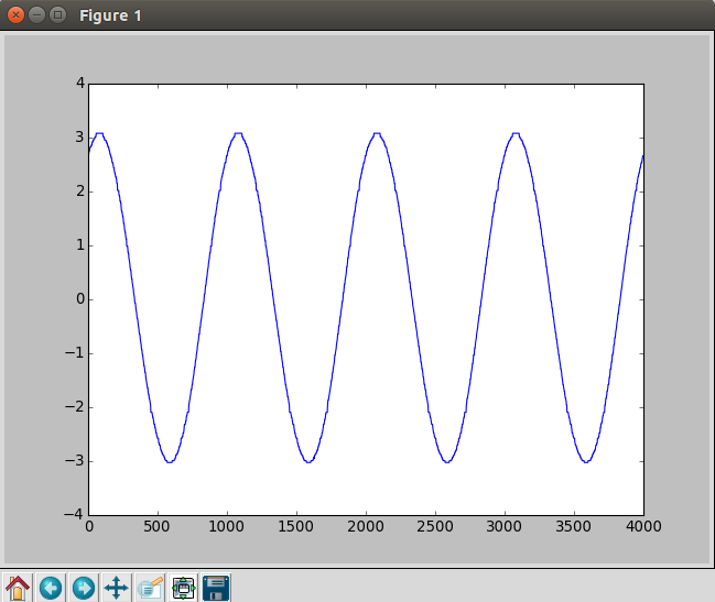
If the same were taken via a script that shares CPU time with other processes, the waveform would compress at random intervals due to CPU time unavailability. Starting a new CPU intensive process usually has the effect of the entire waveform appearing compressed because actual time intervals between each sample are greater than the expected time intervals
Implementing the oscilloscope for data buses such as I2C
With regards to the PSLab which already has a reasonably accurate oscilloscope built-in, what happens if one wants to acquire time critical information from sensors connected to the data bus , and not the analog inputs ?
In order acquire such data , the PSLab firmware houses the read routine from I2C in an interrupt function that is invoked at precise intervals by a preconfigured timer’s timeout event. Each sample is stored to an array via a self incrementing pointer.
The I2C address to be accessed, and the bytes to be written before one can start reading data are all pre-configured before the acquisition process starts.
This process then runs at top priority until a preset number of samples have been acquired.Once the host software knows that acquisition should have completed, it fetches the data buffer containing the acquired information.
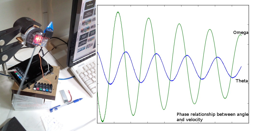
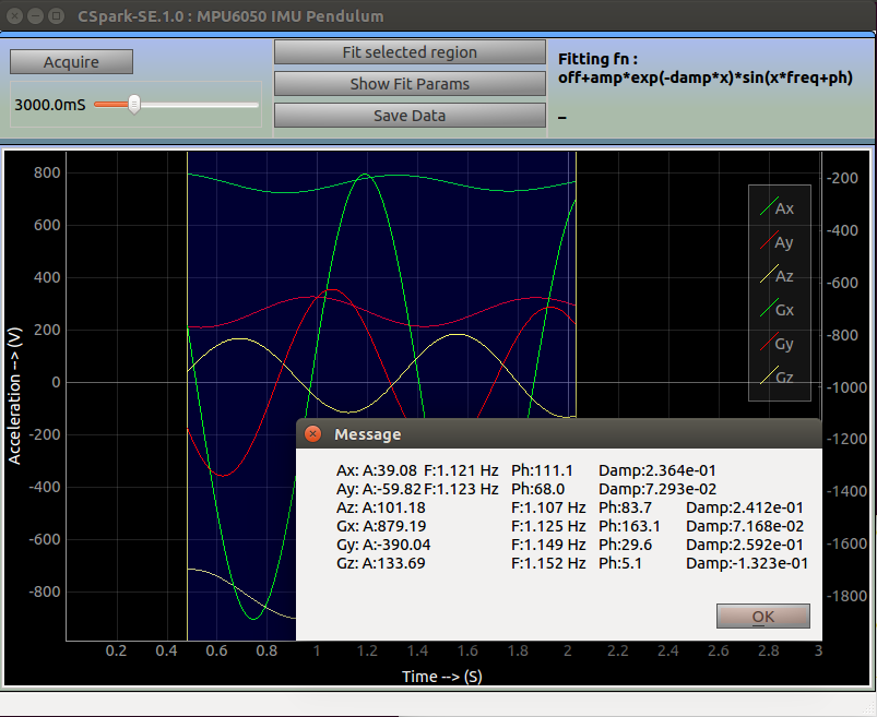
The plots that overlap accurately with a simulated damped sinusoidal waveform are not possible in the absence of a real-time acquisition system
The sensor in question is the MPU6050 from invensense, used primarily in drones, and other self-stabilising robots.
Its default I2C address is 0x68 ( 104 ) , and 14 registers starting from 0x3B contain data for acceleration along orthogonal axes, temperature, and angular velocity along orthogonal axes. Each of these values is an integer, and is therefore represented by two successive registers. E.g. , 0x3B and 0x3C together make up a 16-bit value for acceleration along the X-axis.
The Final App