Implementing Tree View in PSLab Android App

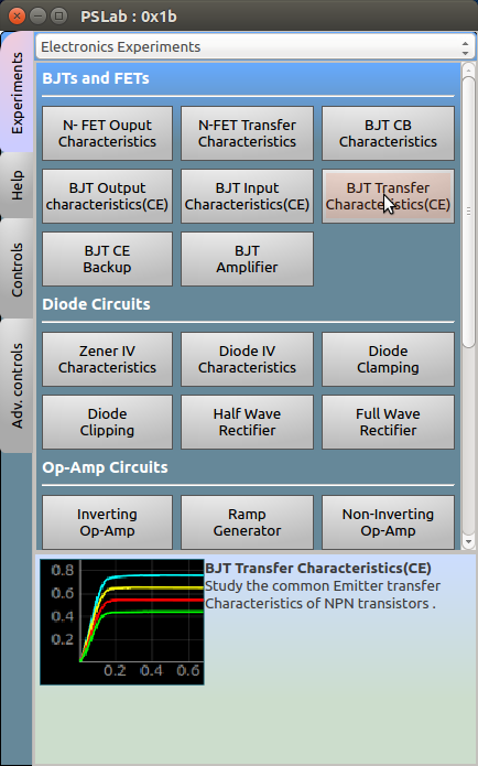
When a task expands over sub tasks, it can be easily represented by a stem and leaf diagram. In the context of android it can be implemented using an expandable list view. But in a scenario where the subtasks has mini tasks appended to it, it is hard to implement it using the general two level expandable list views. PSLab android application supports many experiments to perform using the PSLab device. These experiments are divided into major sections and each experiments are listed under them.

The best way to implement this functionality in the android application is using a multi layer treeview implementation. In this context three layers are enough as follows;


This was implemented with the help from a library called AndroidTreeView. This blog will outline how to modify and implement it in PSLab android application.

Basic Idea

Tree view implementation simply follows the data structure “Tree” used in algorithms. Every tree has a root where it starts and from the root there will be branches which are connected using edges. Every edge will have a parent and child. To reach a child, one has to traverse through only one route.

Setting Up Dependencies

Implementing tree view begins with setting up dependencies in the gradle file in the project.

compile 'com.github.bmelnychuk:atv:1.2.+'

Creating UI for tree view

The speciality about this implementation is that it can be loaded into any kind of a layout such as a linearlayout, relativelayout, framelayout etc.

final TreeNode Root = TreeNode.root();
Root.addChildren(
       // Add child nodes here
);
// Set up the tree view
AndroidTreeView experimentsListTree = new AndroidTreeView(getActivity(), Root);
experimentsListTree.setDefaultAnimation(true);
[LinearLayout/RelativeLayout].addView(experimentsListTree.getView());

Creating a node holder

Trees are made of a collection of tree nodes. A holder for a tree node can be created using an object which extends the BaseNodeViewHolder class provided by the library. BaseNodeViewHolder requires a holder class which is generally static so that it can be accessed without creating an instance which nests textviews, imageviews and buttons.

Once the holder extends the BaseNodeViewHolder, it should override two methods as follows;

@Override
public View createNodeView(final TreeNode node, ClassContainingNodeData header) {

}

@Override
public void toggle(boolean active) {

}

createNodeView() which inflate the view and toggle() method which can be used to toggle clicks on the tree node in the UI.

The following code snippet shows how to create an object which extends the above mentioned class with the overridden methods.

public class ExperimentHeaderHolder extends TreeNode.BaseNodeViewHolder<ExperimentHeaderHolder.ExperimentHeader> {

    private ImageView arrow;

    public ExperimentHeaderHolder(Context context) {
            super(context);
    }

    @Override
    public View createNodeView(final TreeNode node, ExperimentHeader header) {

            final LayoutInflater inflater = LayoutInflater.from(context);
            final View view = inflater.inflate(R.layout.header_holder, null, false);

            TextView title = (TextView) view.findViewById(R.id.title);
            title.setText(header.title);

            arrow = (ImageView) view.findViewById(R.id.experiment_arrow);
        
            return view;
    }

    @Override
    public void toggle(boolean active) {
            arrow.setImageResource(active ? arrow_drop_up : arrow_drop_down);
    }

    public static class ExperimentHeader {

            public String title;

            public ExperimentHeader(String title) {
               this.title = title;
            }
    }
}

Creating a TreeNode

Once the holder is complete, we can move on to creating an actual tree node. TreeNode class requires an object which extends the BaseNodeViewHolder class as mentioned earlier. Also it requires a viewholder which it can use to inflate the view in the tree layout. The viewholder can be a different class. The importance of this different implementation can be explained as follows;

TreeNode treeNode = new TreeNode(new ExperimentHeaderHolder.ExperimentHeader(“Title”))
       .setViewHolder(new ExperimentHeaderHolder(context));

In the Saved Experiments section of PSLab android application, all the three levels shouldn’t implement the toggle behavior as a user clicks on the experiment (last level item), he doesn’t expect the icon to change like the ones in headers where an arrow points up and down when he clicks on it. In this case we can reuse a holder which has the title attribute while creating only a holder which does not override the toggle function to ignore icon toggling at the last level of the tree view. This explanation can be illustrated using a code snippet as follows;

new TreeNode(new ExperimentHeaderHolder.ExperimentHeader(“Title”))
       .setViewHolder(new IndividualExperimentHolder(context));

Creating parent nodes and finally the Root node

The final part of the implementation is to create parent nodes to group up similar experiments together. The TreeNode object supports a method call addChild() and addChildren(). addChild() method allows adding one tree node to the specific tree node and addChildren() method allows adding many tree nodes at the same time. Following code snippet illustrates how to add many tree nodes to a node and make it a parent node.

treeDiodeExperiments.addChildren(treeZener, treeDiode, treeDiodeClamp, treeDiodeClip, treeHalfRectifier, treeFullWave);

Setting a click listener

Click listener is a very important implementation. Each tree node can be attached with a click listener using the interface provided by the library as follows;

treeNode.setClickListener(new TreeNode.TreeNodeClickListener() {
   @Override
   public void onClick(TreeNode node, Object value) {

   }
});

The value object is the class attached to the holder and its attributes can be retireved by casting it to the specific class using casting methods;

String title = ((ExperimentHeaderHolder.ExperimentHeader) value).title;

Resources:

Continue ReadingImplementing Tree View in PSLab Android App

I2C Communication in PSLab

PSLab supports communication using the I2C protocol and both the Desktop App and the Android App have the framework set-up to use the I2C protocol. I2C protocol is mainly used by sensors which can be connected to PSLab. For supporting I2C communication, PSLab board has a separate block for I2C communication and has pins named 3.3V, GND, SCL and SDA. A brief overview of how I2C communication works and its advantages & limitations compared to SPI communication can be found here.

The PSLab Python and Java communication libraries have a class dedicated for I2C communication with numerous methods defined in them. The methods required for a particular I2C sensor may differ, however, in general most sensors utilise a certain common set of methods. The set of methods that are commonly used are listed below with their functions. For utilising the methods, the I2C bus is first notified using the HEADER byte (it is common to all the methods) and then a byte to uniquely determine the method in use.

The send method is used to send the data over the I2C bus. First the I2C bus is initialised and set to the correct slave address using I2C.start(address) followed by this method. The method takes the data to be sent as the argument.

def send(self, data):
    try:
        self.H.__sendByte__(CP.I2C_HEADER)
        self.H.__sendByte__(CP.I2C_SEND)
        self.H.__sendByte__(data)  # data byte
        return self.H.__get_ack__() >> 4
    except Exception as ex:
        self.raiseException(ex, "Communication Error , Function : " + inspect.currentframe().f_code.co_name)


The read method reads a fixed number of bytes from the I2C slave. One can also use I2C.simpleRead(address,  numbytes) instead to read from the I2C slave. This method takes the length of the data to be read as argument.  It fetches length-1 bytes with acknowledge bits for each.

def read(self, length):
     data = []
     try:
        for a in range(length - 1):
             self.H.__sendByte__(CP.I2C_HEADER)
             self.H.__sendByte__(CP.I2C_READ_MORE)
             data.append(self.H.__getByte__())
             self.H.__get_ack__()
       self.H.__sendByte__(CP.I2C_HEADER)
       self.H.__sendByte__(CP.I2C_READ_END)
       data.append(self.H.__getByte__())
       self.H.__get_ack__()
    except Exception as ex:
       self.raiseException(ex, "Communication Error , Function : " + inspect.currentframe().f_code.co_name)
   return data


The readBulk method reads the data from the I2C slave. This takes the I2C slave device address, the address of the device from which the data is to be read and the length of the data to be read as argument and the returns the bytes read in the form of a list.

def readBulk(self, device_address, register_address, bytes_to_read):
        try:
            self.H.__sendByte__(CP.I2C_HEADER)
            self.H.__sendByte__(CP.I2C_READ_BULK)
            self.H.__sendByte__(device_address)
            self.H.__sendByte__(register_address)
            self.H.__sendByte__(bytes_to_read)
            data = self.H.fd.read(bytes_to_read)
            self.H.__get_ack__()
            try:
                return [ord(a) for a in data]
            except:
                print('Transaction failed')
                return False
        except Exception as ex:
           self.raiseException(ex, "Communication Error , Function : " + inspect.currentframe().f_code.co_name)


The writeBulk method writes the data to the I2C slave. It takes address of the particular I2C slave for which the data is to be written and the data to be written as arguments.

def writeBulk(self, device_address, bytestream):
        try:
            self.H.__sendByte__(CP.I2C_HEADER)
            self.H.__sendByte__(CP.I2C_WRITE_BULK)
            self.H.__sendByte__(device_address)
            self.H.__sendByte__(len(bytestream))
            for a in bytestream:
                self.H.__sendByte__(a)
            self.H.__get_ack__()
        except Exception as ex:
  self.raiseException(ex, "Communication Error , Function : " + inspect.currentframe().f_code.co_name)


The scan method scans the I2C port for connected devices which utilise I2C as a communication mode. It takes frequency as an argument to set the frequency of the communication and is by default set to 100000. An array containing the addresses of the connected devices (which are integers) is returned.

def scan(self, frequency=100000, verbose=False):
        self.config(frequency, verbose)
        addrs = []
        n = 0
        if verbose:
            print('Scanning addresses 0-127...')
            print('Address', '\t', 'Possible Devices')
        for a in range(0, 128):
            x = self.start(a, 0)
            if x & 1 == 0:  # ACK received
                addrs.append(a)
                if verbose: print(hex(a), '\t\t', self.SENSORS.get(a, 'None'))
                n += 1
            self.stop()
       return addrs


Additional Sources

  1. Learn more about the principles behind i2c communication https://learn.sparkfun.com/tutorials/i2c
  2. A simple experiment to demonstrate use of i2c communication with Arduino http://howtomechatronics.com/tutorials/arduino/how-i2c-communication-works-and-how-to-use-it-with-arduino/
  3. Java counterpart of the PSLab I2C library https://github.com/fossasia/pslab-android/blob/master/app/src/main/java/org/fossasia/pslab/communication/peripherals/I2C.java

Continue ReadingI2C Communication in PSLab

High School Physics Practicals using PSLab Device

High school physics syllabus includes rather advanced concepts in the world of Physics; namely practicals related to sound, heat, light and electric. Almost all of these practicals are done in physics labs using conventional bulky equipments. Especially the practicals related to electrical and electronics. They use bulky oscilloscopes with complex controls and multimeter with so many controls. PSLab being a sophisticated device which integrates a whole science lab into a 2” by 2” small circuit, these practicals made easy and interesting.

There are several practicals required to be completed by a student before sitting for GCE (Advanced Level) examination. This blog post points out how to perform those experiments using PSLab device and several other tools required without having to use bulky instruments.

  • Calculating internal resistance and EMF of a dry cell

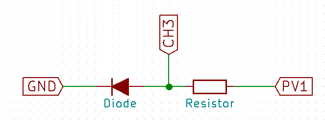
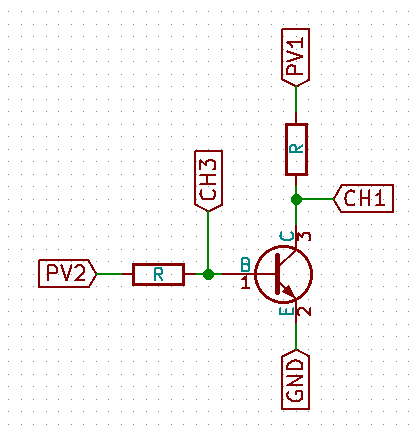
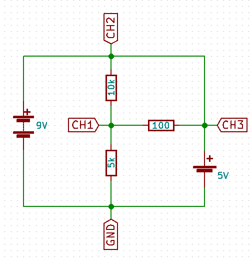
This experiment includes the above mentioned circuitry. Once the basic setup is completed using;
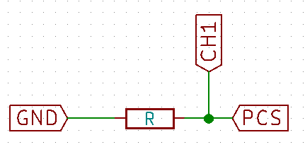
  • Dry cell
  • 10K variable resistor
  • 1K resistor
  • Switch/Jumper

Connect the CH1 pin and GND pin of PSLab across the dry cell and CH2 pin and GND across the Ammeter instead of the Ammeter. Once the pin connection is complete, plug the PSLab device to the computer and using the desktop application voltmeter, measure the voltage from CH1 and current from voltage value read from CH2 and the known resistance value of R. Record these data against step changes in the resistance of the variable resistor starting from a high value to a low value. Once there are sufficient data as much as 10 data set, using a graph paper draw the relation between current and voltage measured according to the equation given below.

E = V + Ir

V = -rI + E

This will produce a graph with a constant negative gradient. Gradient of the graph will produce the internal resistance of the dry cell.

  • I-V graphs for a semiconductor

This experiment will require;

  • Diode
  • 100 Ohms resistor

Conduct the experiment as follows once the circuit is set up. Increase the voltage provided by the PV1 pin of the PSLab by 100 mV per step and measure the voltage across diode using CH3 pin of PSLab device. Using that voltage and the supply voltage, calculate the current flowing through the resistor. Note down the readings as voltage to current pairs and plot them on a graph paper. The graph will produce the following results which is identical to common IV characteristics of a semiconductor.

Start A at zero and increase by 0.1V steps while measuring voltage and current across diode. (Image from Wikipedia)

Apart from this conventional experiment, PSLab provides an inbuilt experiment students and teachers can use. In the Electronics Experiments section, Diode IV characteristics experiment is configured in such a way that this experiment can be conducted very easily. The circuit configuration is the same and R value should be 1K. Once the step size is set to an appropriate resolution, START button will begin the experiment and provide with the final graph.

  • Transfer characteristics of a transistor

Set up the above mentioned circuitry on a breadboard and connect the appropriate pins of PSLab device as mentioned. In this experiment, student need to observe the increase in current/voltage across CH1 when PV2 is varying. We need to measure CH1 parameter value against PV2 voltage value and plot these two against to obtain the transfer characteristics of a BJT.

Apart from this conventional experiment, PSLab provides an inbuilt experiment to perform this lab exercise. Using “BJT Transfer Characteristics” experiment, students and teachers can easily obtain the characteristics curves by setting step sizes and voltage values to the required pins.

  • Ohm’s law

Configure the following circuit and connect PCS, CH1 and GND pins of PSLab into relevant positions. This experiment is to measure voltage across the resistor against the variation in current through the circuit. Increase current provided to the circuit using PCS pin and measure voltage using CH1 pin and plot against the current. The gradient will produce the resistor value.

In the electrical experiments section in PSLab application has a separate experiment to perform the Ohm’s Law experiment. Using this experiment, students can change the current values using the knob and record the voltage values related to that. Finally the plot can be generated which will be of a constant gradient.

  • Kirchhoff’s Laws
  • Voltage law

Kirchhoff’s Voltage law states that the directed sum of the voltage around any closed network is zero.

This law can be proved using the following circuit with the help of PSLab device. Connect the channel pins as per the diagram and measure voltages in the three channels. They will show a relationship as the directed sum of the combination will turn into a zero.

  • Current law

Kirchhoff’s current law states that at any node in a circuit, the sum of currents flowing into that node is equal to the sum of currents flowing out of that node; which is similar to the direct summation of currents in a node is zero.

Using the same circuit as above, measure the current flowing through each node using the voltage readings of the channels and known resistor values. Considering the sign of the current which is easily readable in PSLab desktop application, the summation will produce a zero.

Resources:

Continue ReadingHigh School Physics Practicals using PSLab Device

Characteristization of Transistors Using PSLab

Transistors are one of the key building blocks of all electronics. They are fundamentally three-terminal semiconductor devices, with the terminals being labelled as the Emitter(E), Base(B), and Collector(C). These active components are found everywhere in electronics, and all of the complex processors that power everything from cellphones to aircraft employ millions of these devices in switching and amplification roles. In this blog post, we shall use the PSLab to explore some of the fundamental properties of transistors, and their various applications.

Transistor as an amplifier

In the schematic shown, we shall try to use an NPN transistor to amplify a small signal.

A small amplitude oscillation generated by W1 with the amplitude knob turned down to a very low level is used as the input. Since transistors do not handle bipolar signals, we have mixed a constant DC voltage generated PV3 to shift this small signal into the positive domain.

The fluctuating potential difference incident at the base of the transistor creates a corresponding current flow between the Base and Emitter.

By the fundamental property of transistors, this influences the path resistance between the Collector(C) and the Emitter(E) , and the resultant amplified voltage output can be monitored at the junction between the 1K resistor and the collector.

We have used CH1 to monitor the input voltage, and CH2 for the output

In a more applied scenario, we can implement the second schematic in order to create an audio amplifier. Instead of using W1 as the input signal, a speaker is used as a microphone. When a sound signal is incident on the speaker, its membrane oscillates, and as a result , the coil attached to it also does the same. Since this coil is placed in a magnetic field , its oscillations result in a change in the magnetic flux passing through, and this change causes a voltage(EMF) induced at its output. We then use our transistor amplifier to amplify this small EMF

Figure 2 : A Transistor being used to apply a gain of 81.5x to a small amplitude sine wave. The input waveform (green) is shown on a +/-500mV full scale and the output waveform is shown on a +/-8V scale in order to be able to view both. However, due to the difference in scales, the actual difference in amplitudes is 16 times more than what is visible.
Common Emitter Characteristics
Schematic Diagram

Any introductory course on transistors includes a diagram similar to the one shown , and a description about how for any base current, the collector current eventually saturates, and that this saturation level is proportional to the base current itself.

With the PSLab’s transistor CE characterization app, we can set up this experiment, and verify this for ourselves using an NPN transistor. The results shown were gathered using a 2N2222 transistor

In the schematic , the base current is determined by the voltage source PV2, and a high value series resistor of 200 KOhms . We use an analog input CH3 to monitor the voltage present at the Base of the transistor in order to calculate the total base current.

Base current = V/R = (PV2 – CH3) / 200e3

Now that we have set a particular base current, PV1 is used to sequentially increase the voltage across the collector and emitter of the transistor. A current limiting resistor of 1K Ohm is used, and CH1 is used to monitor the voltage drop across the transistor.

Collector current = V/R = (PV1 – CH1) / 1e3

Plotting the behaviour of the collector current with respect to the collector voltage gives us the familiar current voltage characteristics of a transistor.

Figure 3: Common emitter characteristics of an NPN transistor (2N2222) for various base currents

We can now alter the base current by changing PV2, and verify that the saturation current for the collector is indeed a function of it.

Resources


Continue ReadingCharacteristization of Transistors Using PSLab

Integrating Stock Sensors with PSLab Android App

A sensor is a digital device (almost all the time an integrated circuit) which can receive data from outer environment and produce an electric signal proportional to that. This signal will be then processed by a microcontroller or a processor to provide useful functionalities. A mobile device running Android operating system usually has a few sensors built into it. The main purpose of these sensors is to provide user with better experience such as rotating the screen as he moves the device or turn off the screen when he is making a call to prevent unwanted screen touch events. PSLab Android application is capable of processing inputs received by different sensors plugged into it using the PSLab device and produce useful results. Developers are currently planning on integrating the stock sensors with the PSLab device so that the application can be used without the PSLab device.

This blog is about how to initiate a stock sensor available in the Android device and get readings from it. Sensor API provided by Google developers is really helpful in achieving this task. The process is consist of several steps. It is also important to note the fact that there are devices that support only a few sensors while some devices will support a lot of sensors. There are few basic sensors that are available in every device such as

  • “Accelerometer” – Measures acceleration along X, Y and Z axis
  • “Gyroscope” – Measures device rotation along X, Y and Z axis
  • “Light Sensor” – Measures illumination in Lux
  • “Proximity Sensor” – Measures distance to an obstacle from sensor

The implementing steps are as follows;

  1. Check availability of sensors

First step is to invoke the SensorManager from Android system services. This class has a method to list all the available sensors in the device.

SensorManager sensorManager;
sensorManager = (SensorManager) getSystemService(Context.SENSOR_SERVICE);
List<Sensor> sensors = sensorManager.getSensorList(Sensor.TYPE_ALL);

Once the list is populated, we can iterate through this to find out if the required sensors are available and obstruct displaying activities related to sensors that are not supported by the device.

for (Sensor sensor : sensors) {
   switch (sensor.getType()) {
       case Sensor.TYPE_ACCELEROMETER:
           break;
       case Sensor.TYPE_GYROSCOPE:
           break;
       ...
   }
}

  1. Read data from sensors

To read data sent from the sensor, one should implement the SensorEventListener interface. Under this interface, there are two method needs to be overridden.

public class StockSensors extends AppCompatActivity implements SensorEventListener {

    @Override
    public void onSensorChanged(SensorEvent sensorEvent) {

    }

    @Override
    public void onAccuracyChanged(Sensor sensor, int i) {

    }
}

Out of these two methods, onSensorChanged() method should be addressed. This method provides a parameter SensorEvent which supports a method call getType() which returns an integer value representing the type of sensor produced the event.

@Override
public void onSensorChanged(SensorEvent sensorEvent) {
   switch (sensorEvent.sensor.getType()) {
       case Sensor.TYPE_ACCELEROMETER:
           break;
       case Sensor.TYPE_GYROSCOPE:
           break;
       ...
   }
}

Each available sensor should be registered under the SensorEventListener to make them available in onSensorChanged() method. The following code block illustrates how to modify the previous code to register each sensor easily with the listener.

for (Sensor sensor : sensors) {
   switch (sensor.getType()) {
       case Sensor.TYPE_ACCELEROMETER:
           sensorManager.registerListener(this, sensorManager.getDefaultSensor(Sensor.TYPE_ACCELEROMETER), SensorManager.SENSOR_DELAY_UI);
           break;
       case Sensor.TYPE_GYROSCOPE:
           sensorManager.registerListener(this, sensorManager.getDefaultSensor(Sensor.TYPE_GYROSCOPE), SensorManager.SENSOR_DELAY_UI);
           break;
   }
}

Depending on the readings we can provide user with numerical data or graphical data using graphs plotted using MPAndroidChart in PSLab Android application.

The following images illustrate how a similar implementation is available in Science Journal application developed by Google.

Resources

Continue ReadingIntegrating Stock Sensors with PSLab Android App

Exporting Functions in PSLab Firmware

Computer programs consist of several hundreds line of code. Smaller programs contain around few hundreds while larger programs like PSLab firmware contains lines of code expanding over 2000 lines. The major drawback with a code with lots of lines is the difficulty to debug and hardship for a new developer to understand the code. As a solution modularization techniques can be used to have the long code broken down to small set of codes. In C programming this can be achieved using different .c files and relevant .h(header) files.

The task is tricky as the main code contains a lot of interrelated functions and variables. Lots of errors were encountered when the large code in pslab-firmware being modularized into application specific files. In a scenario like this, global variables or static variables were a much of a help.

Global Variables in C

A global variable in C is a variable whose scope spans wide across the entire program. Updation to the variable will be reflected everywhere it is used.

extern TYPE VARIABLE = VALUE;

Static Variables in C

This type of variables preserve their content regardless of the scope they are in.

static TYPE VARIABLE = VALUE;

Both the variables preserve their values but the memory usage is different depending on the implementation. This can be explained using a simple example.

Suppose a variable is required in different C files and it is defined in one of the header files as a local variable. The header file is then added to several other c files. When the program is compiled the compiler will create several copies of the same variable which will throw a compilation error as variable is already declared. In PSLab firmware, a variable or a method from one library has a higher probability of it being used in another one or many libraries.

This issue can be addressed in two different ways. They are by using static variables or global variables. Depending on the selection, the implementation is different.

The first implementation is using static variables. This type of variables at the time of compilation, create different copies of himself in different c files. Due to the fact that C language treats every C file as a separate program, if we include a header file with static variables in two c files, it will create two copies of the same variable. This will avoid the error messages with variables redeclared. Even though this fixes the issue in firmware, the memory allocation will be of a wastage. This is the first implementation used in PSLab firmware. The memory usage was very high due to duplicate variables taking much memory than they should take. This lead to the second implementation.

first_header.h

#ifndef FIRST_HEADER_H 
#define FIRST_HEADER_H 

static int var_1;

#endif 

/* FIRST_HEADER_H */

second_header.h

#ifndef SECOND_HEADER_H
#define SECOND_HEADER_H

static int var_1;

#endif    

/* SECOND_HEADER_H */

first_header.c

#include <stdio.h>
#include "first_header.h"
#include "second_header.h"

int main() {
    var_1 = 10;
    printf("%d", var_1);
}

The next implementation uses global variables. This type of variables need to be declared only in one header file and can be reused by declaring the header file in other c files. The global variables must be declared in a header file with the keyword extern and defined in the relevant c file once. Then it will be available throughout the application and no errors of variable redeclaration will occur while compiling. This became the final implementation for the PSLab-firmware to fix the compilation issues modularizing application specific C and header files.

Resources:

Continue ReadingExporting Functions in PSLab Firmware

Understanding PN Junctions with the Pocket Science Lab

The boundary layer between two thin films of a semiconducting material with Positive type and Negative type doping is referred to as a P-N junction, and these are one of the fundamental building blocks of electronics. These junctions exhibit various properties that have given them a rather indispensable status in modern day electronics.

The PSLab’s various measurement tools enable us to understand these devices, and in this blog post we shall explain some uses of PN junctions, and visualize their behaviour with the PSLab.

One might easily be confused and assume that a positive doping implies that the layer has a net positive charge, but this is not the case. A positive doping involves replacing a minute quantity of the semiconductor molecules with atoms from the next column in the periodic table. These atoms such as phosphorus are also charge neutral, but the number of available mobile charge carriers effectively increases.

A diode as a half-wave rectifier

A diode is basically just a PN junction. An ideal diode conducts electricity in one direction offering a path of zero resistance, and it is a perfect insulator in the other direction. In practice, we may observe some additional properties.

Figure : The circuit used for making the half-wave rectifier and studying it. A bipolar sinusoidal signal is input to a diode, and the output voltage is monitored. The 1uF capacitor is used to filter the output signal and make it more or less constant, but it has not been used while obtaining the data shown in the following image

Figure : A diode used as a half-wave rectifier. The input waveform shown in green was passed through a forward biased diode, and monitored by CH2 (red trace ) .

We can observe that only the positive half of the signal passes through the diode. It can also be observed , that since this is not an ideal diode, the conducted portion has lost some amplitude. This loss is a consequence of the forward threshold voltage of the PN junction, and in case of this diode, it is around 0.6 Volts. This threshold voltage depends on the band structure of the diode , and in the next section we shall examine this voltage for various diodes.

Measurement of Current-Voltage Characteristics of diodes

In practice, diodes only start conducting in the forward direction after a certain threshold potential difference is present. This voltage, also known as the barrier potential, depends on the band gap of the diode, and we shall measure it to determine how the electrical properties affect the externally visible physical properties of the diode.

A programmable voltage output of the PSLab (PV1) will be increased in small steps starting from 0 Volts, and a voltmeter input (CH3) will be used to determine the point when the diode starts conducting. The presence of a known resistor between PV1 and CH3 acts as a current limiter, and also enables us to calculate the current flow using some elementary application of the Ohm’s law. I = (PV1-CH3)/1000 .


The following image shows I-V characteristics of various diodes ranging from Schottky to Light Emitting Diodes (LEDs).

It may be interesting to note that the frequency of the light emitted by LEDs is directly proportional to the threshold voltage. In case of the white LED, it is almost similar to the blue LED because white LEDs are composed of blue LEDs, and a phosphor coating that partially converts blue light to yellow. The combination results in white light.

Zener diodes

Zener diodes are a special variant of diodes that also conduct electricity in the the reverse direction once a certain threshold has been crossed. This threshold can be determined during the manufacturing process, and zener diodes with breakdown voltages such as 3.3V , 5.6V , 6.8V etc are commercially available.

In the following image, the I-V characteristics of a 3.3V zener diode have been measured with the PSLab . As can be observed, the diode starts to conduct small amounts of current from around 2V itself, but significant current flow is usually present once the rated voltage is achieved.

In the forward direction, the zener appears to behave as a regular diode.

Resources

Continue ReadingUnderstanding PN Junctions with the Pocket Science Lab

Real time Sensor Data Analysis on PSLab Android

PSLab device has the capacity to connect plug and play sensors through the I2C bus. The sensors are capable of providing data in real time. So, the PSLab Android App and the Desktop app need to have the feature to fetch real time sensor values and display the same in the user interface along with plotting the values on a simple graph.

The UI was made following the guidelines of Google’s Material Design and incorporating some ideas from the Science Journal app. Cards are used for making each section of the UI. There are segregated sections for real time updates and plotting where the real time data can be visualised. A methods for fetching the data are run continuously in the background which receive the data from the sensor and then update the screen.

The following section denotes a small portion of the UI responsible for displaying the data on the screen continuously and are quite simple enough. There are a number of TextViews which are being constantly updated on the screen. Their number depends on the type and volume of data sent by the sensor.

<TextView
       android:layout_width="wrap_content"
       android:layout_height="30dp"
       android:layout_gravity="start"
       android:text="@string/ax"
       android:textAlignment="textStart"
       android:textColor="@color/black"
       android:textSize="@dimen/textsize_edittext"
       android:textStyle="bold" />

<TextView
       android:id="@+id/tv_sensor_mpu6050_ax"
       android:layout_width="wrap_content"
       android:layout_height="30dp"
       android:layout_gravity="start"
       android:textAlignment="textStart"
       android:textColor="@color/black"
       android:textSize="@dimen/textsize_edittext"
       android:textStyle="bold" />


The section here represents the portion of the UI responsible for displaying the graph. Like all other parts of the UI of PSLab Android, MPAndroidChart is being used here for plotting the graph.

<LinearLayout
       android:layout_width="match_parent"
       android:layout_height="160dp"
       android:layout_marginTop="40dp">

       <com.github.mikephil.charting.charts.LineChart
               android:id="@+id/chart_sensor_mpu6050"
               android:layout_width="match_parent"
               android:layout_height="match_parent"
               android:background="#000" />
</LinearLayout>


Since the updates needs to continuous, a process should be continuously run for updating the display of the data and the graph. There are a variety of options available in Android in this regard like using a Timer on the UI thread and keep updating the data continuously, using ASyncTask to run a process in the background etc.

The issue with the former is that since all the processes i.e. fetching the data and updating the textviews & graph will run on the UI thread, the UI will become laggy. So, the developer team chose to use ASyncTask and make all the processes run in the background so that the UI thread functions smoothly.

A new class SensorDataFetch which extends AsyncTask is defined and its object is created in a runnable and the use of runnable ensures that the thread is run continuously till the time the fragment is used by the user.

scienceLab = ScienceLabCommon.scienceLab;
i2c = scienceLab.i2c;
try {
    MPU6050 = new MPU6050(i2c);
} catch (IOException e) {
    e.printStackTrace();
}
Runnable runnable = new Runnable() {
    @Override
    public void run() {
        while (true) {
            if (scienceLab.isConnected()) {
                try {
                    sensorDataFetch = new SensorDataFetch();
                } catch (IOException e) {
                    e.printStackTrace();
                }
                sensorDataFetch.execute();
            }
        }
    }
};
new Thread(runnable).start();


The following is the code for the ASyncTask created. There are two methods defined here doInBackground and onPostExecute which are responsible for fetching the data and updating the display respectively.

The raw data is fetched using the getRaw method of the MPU6050 object and stored in an ArrayList. The data type responsible for storing the data will depend on the return type of the getRaw method of each sensor class and might be different for other sensors. The data returned by getRaw is semi-processed and the data just needs to be split in sections before presenting it for display.

The PSLab Android app’s sensor files can be viewed here and they can give a better idea about how the sensors are calibrated, how the intrinsic nonlinearity is taken care of, how the communication actually works etc.

After the data is stored, the control moves to the onPostExecute method, here the textviews on the display and the chart are updated. The updation is slowed down a bit so that the user can visualize the data received.

private class SensorDataFetch extends AsyncTask<Void, Void, Void> {
   MPU6050 MPU6050 = new MPU6050(i2c);
   ArrayList<Double> dataMPU6050 = new ArrayList<Double>();

   private SensorDataFetch(MPU6050 MPU6050) throws IOException {
   }

   @Override
   protected Void doInBackground(Void... params) {
       try {
           if (MPU6050 != null) {
               dataMPU6050 = MPU6050.getRaw();
           }
       } catch (IOException e) {
           e.printStackTrace();
       }
           return null;
   }

   protected void onPostExecute(Void aVoid) {
       super.onPostExecute(aVoid);
       tvSensorMPU6050ax.setText(String.valueOf(dataMPU6050.get(0)));
       tvSensorMPU6050ay.setText(String.valueOf(dataMPU6050.get(1)));
       tvSensorMPU6050az.setText(String.valueOf(dataMPU6050.get(2)));
       tvSensorMPU6050gx.setText(String.valueOf(dataMPU6050.get(3)));
       tvSensorMPU6050gy.setText(String.valueOf(dataMPU6050.get(4)));
       tvSensorMPU6050gz.setText(String.valueOf(dataMPU6050.get(5)));
       tvSensorMPU6050temp.setText(String.valueOf(dataMPU6050.get(6)));
   }
}

The detailed implementation of the same can be found here.

Additional Resources

  1. Learn more about how real time sensor data analysis can be used in various fields like IOT http://ieeexplore.ieee.org/document/7248401/
  2. Google Fit guide on how to use native built-in sensors on phones, smart watches etc. https://developers.google.com/fit/android/sensors
  3. A simple starter guide to build an app capable of real time sensor data analysis http://developer.telerik.com/products/building-an-android-app-that-displays-live-accelerometer-data/
  4. Learn more about using AsyncTask https://developer.android.com/reference/android/os/AsyncTask.html

Continue ReadingReal time Sensor Data Analysis on PSLab Android

Using Hierarchical Blocks in KiCAD to Collaborate in PSLab Hardware Development

The PSLab hardware project designed in KiCAD, an ECAD tool; doesn’t support collaborative features like Git providing for software projects. As explained in a previous blog post on techniques to help up with project collaboration, this blog post will demonstrate how two developers can work together on the same hardware project.

The difficulties arise as the whole project is in one big schematic file. Editing made by one developer will affect to the editing done by the other developers causing merge conflicts. KiCAD doesn’t compile nicely if the changes were fixed manually most of the cases.

The solution practiced in the pslab-hardware project is using hierarchical blocks. This blog post will use a KiCAD project with an oscillator implementation and a voltage regulator implementation just like the ones in pslab-hardware schematics. To avoid complications in understanding changes in a huge circuit, only these two modules will be implemented separately in the blog.

Initially the project will look like the following figure;

Sheet1 Sheet2

These two hierarchical blocks will be created as different .sch files in the project directory as follows;

Assume two different developers are working on these two different blocks. That is the key concept in collaborating hardware projects in KiCAD. As long as the outer connections (pins) don’t get changed, edits made to one block will have no effect on the other blocks.

Developer 1 decided that the existing power circuit is not efficient for the PSLab device. So he decided to change the circuit in Sheet 1. The circuit before and after modification is shown in the table below.

Sheet 1 (Before) Sheet 1 (After)

If we take a look at the git status now, it will be as follows;

From this it is noticeable that neither the main schematic file nor Developer2.sch hasn’t been touched by the edits made to Developer1.sch file. This avoids merge conflicts happening when all the developers are working on the same schematic file.

Resources :

Continue ReadingUsing Hierarchical Blocks in KiCAD to Collaborate in PSLab Hardware Development

How to Read PIC Data-Sheet and Add a New Functionality to PSLab Firmware

Reading data-sheets is not a fun task. Going through tens of hundreds of pages with numerical, mathematical and scientific data is not fun reading. This blog post attempts to simplify reading the available data-sheets related to PIC24 micro-controller used in the PSLab device to help reader with implementing a new feature in PSLab firmware.

There are many features available in the PSLab device, such as; UART, SPI, I2C, ADC and Basic I/O reading. The “basic” implementation techniques do not vary much from one feature to other. That being stated this blog will carry out the basic implementation techniques one should follow and basic knowledge on PIC micro-controller programming to save himself from the trouble going through the 500+ pages in PIC data-sheets.

PIC Basics:

Before go into implementation there are few facts one should know about PIC programming.

– In the micro-controller values are saved in a memory block known as Registers. The values saved in these registers are volatile as they are all set to 0 regardless the value they were assigned when the power is off.

– Micro-controller configurations are made by setting values to these registers. Even turning on and off a whole feature like UART in PSLab device can be done using setting 0 to UARTEN register bit.

– When it comes to I/O ports, there are two different types of registers called TRIS and LAT/PORT. By setting 1 to TRIS ports will make the relevant pin an input pin. Setting it to 0 will make it an output pin. Easy way to remember this is think 1 as I in input and 0 as O in output. In UART implementation of PSLab, pin RP40 is set as an input pin to receive the data stream and pin RP39 is set as an output pin to send the data stream out. These settings are made using TRIS port settings. PORT registers save the value received by the relevant input pin attached to it.


The above figure extracted from mikroe learning materials, illustrates different stages an I/O pin can handle. As an extra point, ANSEL register makes the pin support digital signals or analog signals as per user requirements.

– In PIC, some registers such as PORT, TRIS and registers with similar functionalities are combined together. To access the value of each individual register can be done using dot notation. Assume the program requires to access the 8th register in TRISB register set. Note that the registers are indexed from zero. This implies that the 8th register will have the index 8 in the register sub-set. The following syntax is used to access the register;

TRISBbits.TRISB7


The above points cover the basic knowledge one should have when developing firmware to PSLab device.

How to implement a feature like UART in PSLab firmware?

The first thing to know when implementing a new feature is that the developer needs to be familiar with the relevant hardware protocols. As an example, to implement UART; relevant protocol is RS232. If the feature is I2C; one should know about the I2C protocol.

Once the feature is familiar, next step is to refer the PIC data-sheet and resources on how to implement it in firmware. As for demonstrative purposes, this blog will continue with UART implementation.

Download the latest data-sheet from MicroChip official website and browse to the table of content. It consists of a set of features supported by the micro-controller implemented in the PSLab device. Find the entry related to the feature being implemented. In this case it will be Universal Asynchronous Receiver Transmitter (UART).

Each feature will contain a description following this format explaining what are the options it support and its constraints.

One must be aware of the fact that not every pin in the micro-controller can be used for any feature as he desires. The “PINOUT I/O DESCRIPTIONS” section in the data-sheet explains which pins are capable of the feature being implemented. According to these details, the pins should be initiated as Input/Output pins as well as Digital/Analog pins.

The next step is to refer to the control registers related to the feature. They are all mentioned in the data-sheet under the specific feature. There are some notations available in this section which resembles something like the following;

PDSEL<1:0>: Parity and Data Selection bits
11 = 9-bit data, no parity
10 = 8-bit data, odd parity
01 = 8-bit data, even parity
00 = 8-bit data, no parity


This represents a register with two bits. By setting either 11 or 10 or 01 or 00; different implementations can be achieved.

In PSLab firmware this is implemented as;

U1MODEbits.PDSEL = 0;


which implements UART feature with 8-bits stream having no parity bits for error correction.

In UART feature implemented in PSLab device, receiving bit stream is fetched by reading the register values in U1STAbits.URXDA and data is transmitted using U1TXREG. All these registers are mentioned in the control registers section in the feature.

Resources:

Continue ReadingHow to Read PIC Data-Sheet and Add a New Functionality to PSLab Firmware