Measuring CO2 with MQ135

Introduction

A MQ135 sensor on a small PCB.

The MQ135 is a cheap gas sensor that is primarily intended for detecting the presence of flammable gases. It is marketed as a generalized “air quality” sensor, rather than precision device for measuring the concentration of any specific gas. Nevertheless, according to the data sheet the MQ135 is capable of measuring the concentrations of several gases, one of which is CO2. This makes it an attractive low-cost alternative to more specialized (and more expensive) CO2-specific sensors.

Much has been written about using the MQ135 as a CO2 sensor, mostly focusing on using it together with Arduino. This article will, firstly, discuss the working principles of the MQ135 sensor and how to read the data sheet, and secondly present how to use it with the PSLab.

Theory of operation

The MQ135 consists of a surface covered in a thin layer of SnO2, and a heater resistor which serves to raise the temperature of the SnO2 surface to several hundred degrees Celsius. SnO2 is an n-type semiconductor, in which donor electrons are excited to the conduction band at elevated temperatures. However, SnO2 when exposed to air readily adsorbs oxygen onto its surface. The adsorption reaction consumes electrons from the conduction band to form negatively charged oxygen species. Therefore, SnO2 has low conductivity in clean air. [Shimizu]

In the presence of a flammable gas, the gas will also adsorb onto the sensor surface, where it consumes the adsorbed oxygen species to form CO2 and H2O. This reaction releases the donor electrons back into the conduction band, thereby raising the conductivity of the sensor. By quantifying the conductivity response to the presence of various gases, a thin SnO2 surface can be used to determine the concentration of the gas. [Shimizu]

CO2, notably, is not a flammable gas. Here, the sensing mechanism is different; instead of reacting with adsorbed oxygen directly, CO2 sensing relies on water vapor first reacting with adsorbed oxygen to form adsorbed hydroxide (OH). CO2 then in turn reacts with the adsorbed hydroxide, forming carbonate (CO32-). This process ultimately also returns electrons to the SnO2 conduction band, and therefore results in increased conductivity. [Wang et al.]

SnO2 gas sensors can also detect the presence of reducing gases such as NOx. Here, the sensing mechanism is the opposite; the reducing gas adsorbs onto the sensor surface, consuming additional electrons from the conduction band, and thereby lowers the conductivity further. The MQ135 data sheet does not specify response curves for any reducing gases, so while the sensor should be sensitive to such gases, the user would have to experimentally determine the response curves themselves. [Shimizu]

MQ135 gas response curves

The MQ135 data sheet provides a graph showing how the sensor resistance changes with the concentration of several gases. Figure 1 shows a reproduction of the data sheet graph, where the points have been manually extracted from the data sheet graph using WebPlotDigitizer.

Note that the y-axis is Rs/R0, which is the ratio between the sensor resistance at any given moment (Rs) and the sensor resistance at a specific set of conditions (R0). This is because the sensor resistance depends on the exact amount of active material on the sensor surface, which varies between individual sensors. Therefore, the resistance response must be normalized against a predefined state in order for results from different sensors to be comparable. For the MQ135, this predefined state is 100 ppm ammonia vapor in otherwise clean air at 20 °C and 65% relative humidity. The sensor resistance at this state must be known in order for the curves in Figure 1 to apply. This may seem like a problem, since most people will not be able to reproduce those conditions. Fortunately, there are other ways to derive R0. More on that later.

The responses show clearly linear behavior in loglog-scale, which means that the relationship between resistance and concentration can be expressed as:

RS / R0 = a * cb    (1)

where a and b are constants, and c is gas concentration in ppm.

The curves in the Figure 1 have been fitted using exponential regression, specifically scipy.optimize.curve_fit.

Figure 2: Data sheet gas response values (points) and fitted curves (lines).

Equation 1 gives the sensor resistance as a function of gas concentration, but we are interested in the opposite relation, i.e. gas concentration as a function of sensor resistance. A little elementary algebra gets us there:

c = (1 / a)1/b * (RS / R0)1/b = A * (RS / R0)B    (2)

With that, we can correlate sensor resistance with gas concentration for any of the gases in Figure 1. Now, we need a way to determine the sensor resistance.

MQ135 electrical characteristics

As previously mentioned, the MQ135 behaves as a variable resistor when exposed to different gas concentrations. In order to measure gas concentration using equation 2, we need a way to measure the sensor resistance.

Figure 3: Circuit diagram of a typical sensing circuit using a MQ135. Note the voltage divider in the upper path.

By connecting a resistor in series with the sensor and measuring the voltage between them we can create a voltage divider, as in figure 3. The expression for the output voltage from a voltage divider is:

Vout = RL / (RS + RL) * Vin    (3)

Rearrange to isolate the sensor resistance:

RS = RL * (Vin / Vout – 1)    (4)

Understanding R0

While equation 4 provides a way to measure the sensor resistance, the sensor resistance alone is not enough to determine the gas concentration. This is because every individual sensor has a unique resistance response, based on the amount and distribution of active material on the sensor surface. Therefore, in order to compare the response of one sensor with other sensors, the response must be normalized. R0 is the normalization factor, and is defined as the sensor resistance at a known set of conditions, i.e. a certain temperature, relative, humidity, and most importantly a certain gas concentration. The ratio of the sensor resistance and R0 can be compared between sensors.

The MQ135 data sheet defines R0 as the sensor resistance at 100 ppm ammonia at 20 °C and 65% relative humidity. Of course, it is possible to redefine R0 at some other set of conditions, but if R0 is redefined, the curves in Figure 2 no longer apply! The only situation where it makes sense to redefine R0 is if you have the means to create new response curves for the gas you wish to measure. Otherwise, keeping R0 defined as above is the best available option.

That means we need a way to calculate R0, since most people will not be able to recreate the conditions at which it is defined. By rearranging equation 2, we get:

R0 = RS * (1 / A * c)-1/B    (5)

Since we can measure the sensor resistance, that means the only unknown term in the RHS of equation 5 is the concentration. In other words, if we can measure the sensor resistance in any known gas concentration, we can calculate R0.

As it happens, we do know the concentration of one of the gases in figure 2: Carbon dioxide. The concentration of CO2 in outside air is around 400 ppm (and rising, check co2.earth for up to date values if you are reading this some years after 2021).

Accounting for temperature and humidity

The sensor response also depends on ambient temperature and humidity. The data sheet specifies the effect on sensor response at four different temperatures and two different humidity levels for ammonia vapor. Figure 4 shows a reproduction of the data sheet graph, plus fitted curves.

Figure 4: Data sheet temperature / humidity corrections (points) and fitter curves (lines).

From figure 4 we can see that the sensor resistance reaches a minimum at some temperature TM and then starts to increase. The reason the resistance decreases as the temperature increases toward TM is that higher surface temperature contributes to faster reaction rates between the gas and the adsorbed oxygen. The increase in sensor resistance at temperatures above TM can be explained by faster re-adsorption of oxygen at higher temperatures, which means more oxygen will cover the sensor surface for the same flammable gas concentration. [Shimizu]

We can also see that sensor resistance seems to decrease with at higher relative humidity. The mechanism for this is less clear. On the one hand, water vapor can adsorb onto the sensor surface, thereby decreasing the oxygen coverage and increasing sensor conductivity. On the other hand, water vapor can heal defective adsorption sites, which increases the surface area available for oxygen adsorption and therefore decreases sensor conductivity. [Wicker et al.] Additionally, recall that the CO2 sensing mechanism is highly dependent on the presence of water. Wang et al. reports a non-linear sensor response to CO2 with respect to humidity, with a response peak at 34% RH. With that in mind, the data sheet humidity dependence graph (which only has two data points and therefore must be assumed to be linear) is of limited utility when measuring CO2.

With that, we have all the pieces we need to use the MQ135 to measure CO2 concentration. Or any other of the gases in figure 2, for that matter. Enough theory, let’s take a look at how to do it in practice using the Pocket Science Lab!

Using the MQ135 with PSLab

If you have just the sensor itself, connect it as shown in figure 5, where the sensor is represented by a SparkFun gas sensor breakout board. CH1 is used to monitor the output voltage of the voltage divider between the sensor and the load resistor (which is 22K in this exaple circuit). Additionally, CH2 is used to monitor the voltage level of the PSLab’s +5V line. It is important that the voltage on the +5V line does not drop below 4.9 V, as the MQ135 will not reach its operating temperature otherwise. The MQ135 heater resistor draws up to 200 mA of current, which may be more power than the USB port powering the PSLab can supply. The PSLab does not regulate the +5V line, so it is up to the USB port to deliver enough current.

Figure 5: Guide to connect MQ135 to PSLab.
Figure 6: A MQ135 mounted on a PCB with a built-in load resistor (highlighted in red), as well as some other circuitry.

If you are using a SNS-MQ135 board, shown in figure 6, simply connect the AO pin to CH1, without the external load resistor. The SNS-MQ135 has its own load resistor, which unfortunately is only 1K. Such a small load resistor means the output voltage on AO will be very small when measuring CO2, which limits measurement accuracy. If possible, you should desolder the built-in SNS-MQ135 load resistor (outlined in red in figure 6), and use an external load resistor as in figure 5 instead. The caveat about the +5V level also applies to the SNS-MQ135.

The MQ135 must be allowed to heat to its operating temperature before it can be used. The data sheet recommends a heating period of at least 24h before use. Additionally, if the sensor hasn’t been used for a long time (or ever, if it is new), it must be allowed to burn in for even longer (>72h) in order to burn off various substances which have reacted with the surface during that time.

After the MQ135 has been allowed to heat up and burn in properly, we can use pslab-python 2.1.0+ to measure the ambient CO2 concentration.

Start by creating a multimeter to measure the voltage level on the +5V line:

>>> import pslab
>>> multimeter = pslab.Multimeter()
>>> multimeter.measure_voltage(“CH2”)
4.961014

If the voltage is at least 4.9 V, the next step is to determine the sensor’s R0. It is a good idea to use an average value over a period of time (this only needs to be done once for each sensor):

>>> import time
>>> from pslab.external.gas_sensor import MQ135
>>> mq135 = MQ135(gas=”CO2”, r_load=22e3)
>>> r0 = []
>>> for i in range(3600):
>>>     r0.append(mq135.measure_r0(400))
>>>     time.sleep(1)
>>> mq135.r0 = sum(r0) / len(r0)

Finally:

>>> mq135.measure_concentration()
418.067514310052683

Done!

References

Shimizu Y. (2014) SnO2 Gas Sensor. In: Kreysa G., Ota K., Savinell R.F. (eds) Encyclopedia of Applied Electrochemistry. Springer, New York, NY. https://doi.org/10.1007/978-1-4419-6996-5_475

Wang et al. (2016) CO2-sensing properties and mechanism of nano-SnO2 thick-film sensor, Sensors and Actuators B: Chemical, Volume 227, Pages 73-84, ISSN 0925-4005, https://doi.org/10.1016/j.snb.2015.12.025

Wicker et al. (2017) Ambient Humidity Influence on CO Detection with SnO2 Gas Sensing Materials. A Combined DRIFTS/DFT Investigation, The Journal of Physical Chemistry C, Volume 121, Number 45, Pages 25064-25073, https://doi.org/10.1021/acs.jpcc.7b06253

Continue ReadingMeasuring CO2 with MQ135

pslab-python 2.0 Release Notes

pslab-python 2.0 is now available! Get it from PyPI or Github.

Large parts of pslab-python have been rewritten to improve user friendliness. pslab-python version 1.0 was written primarily as a back end for pslab-desktop. While it could be used as a standalone library, it was not designed with that use case foremost in mind.

pslab-python 2.0 still serves as the back end for pslab-desktop, but it has been rewritten to be more user-friendly when being used as a standalone library.

Also worth mentioning is pslab-python’s new test suite. Although tests are not immediately useful for users, they help developers avoid accidentally introducing regressions, which in turn makes pslab-python more pleasant to use.

The rewrite touches almost every part of pslab-python and is too extensive to go into detail, so here are the most important user-facing improvements:

Highlights

General

  • Package renamed from PSL to pslab.
  • Simplified API.
  • Improved documentation now available on readthedocs.
  • pslab-python now has a command line interface. Type pslab --help in a terminal for more information.
  • pslab-python can now be installed from PyPI: pip install pslab
  • Reworked exception handling. Exceptions are now raised as soon as possible instead of being suppressed and allowed to propagate.
  • Many, many bug fixes.

Oscilloscope

  • Oscilloscope-related functionality can now be found in the Oscilloscope class.
  • The many different capture methods (capture1, capture2, capture4, capture_multiple, capture_fullspeed, capture_fullspeed_hr, capture_traces, capture_highres_traces) have been combined into a single capture method.
  • Trigger settings can optionally be configured directly in the capture call, without the need to call configure_trigger separately.

Logic Analyzer

  • Logic analyzer-related functionality can now be found in the LogicAnalyzer class.
  • The many different capture methods (capture_edges1, start_one_channel_LA, start_two_channel_LA, start_three_channel_LA, start_four_channel_LA, start_one_channel_LA_backup__) have been combined into a single capture method.
  • The type of logic event to capture is now given as a string instead of a number (e.g. “falling” instead of 2 to capture only falling edges).

Multimeter

  • Multimeter-related functionality can now be found in the Multimeter class.
  • Several different methods for measuring capacitance (capacitance_via_RC_discharge, get_capacitor_range, get_capacitance) have been combined into measure_capacitance.
  • New calibrate_capacitance method added, which allows for measurement of very small (single picofarad) capacitors.

Waveform Generator

  • Analog waveform-related functionality can now be found in the WaveformGenerator class.
  • The many different methods for generating waveforms (set_wave, set_sine1, set_sine2, set_w1, set_w2, set_waves) have been combined into a single generate method.
  • Waveform amplitude is now set directly as part of a loaded function.

PWM Generator

  • PWM-related functionality can now be found in the PWMGenerator class.
  • Several different methods for generator PWM signals (sqr1, sqr1_pattern, sqr2, set_sqrs, sqrPWM) have been combined into a single generate method.

Power Supply

  • Power supply-related functionality can now be found in the PowerSupply class.
  • Voltage and current are now set via properties, e.g. to set the voltage on pin PV1 to 3 V, write power_supply.pv1 = 3.
  • The load resistance limitation on PCS is now clearly documented.

I2C

  • The I2C class has been split into the I2CMaster and I2CSlave classes.
  • Primitive I2C calls (start, stop, wait, restart, etc.) are no longer available. Instead, use read and write which take care of I2C session handling under the hood.

Known issues

  • Not every part of pslab-python has been rewritten. Specifically, the external subpackage (previously known as SENSORS) contains many sensor classes which remain untested.
Continue Readingpslab-python 2.0 Release Notes

Using external UART modules to debug PSLab operations

Pocket Science Lab by FOSSASIA is a compact tool that can be used for circuit analytics and debugging. To make things more interesting, this device can be accessed via the user interface using an Android app or also a desktop app. Both these apps use the UART protocol (Universal Asynchronous Receiver-Transmitter) to transmit commands to the PSLab device from mobile phone or PC and receive commands vice versa. The peculiar thing about hardware is that the developer cannot simply log data just like developing and debugging a software program. He needs some kind of an external mechanism or a tool to visualize those data packets travelling through the wires.

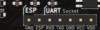
Figure 1: UART Interface in PSLab

PSLab has a UART interface extracted out simply for this reason and also to connect external sensors that use the UART protocol. With this, a developer who is debugging any of the Android app or the desktop app can view the command and data packets transmitted between the device and the user end application.

This  requires some additional components. UART interface has two communication related pins: Rx(Receiver) and Tx(Transmitter). We will need to monitor both these pin signals for input and output data packets. It should be kept in mind that PSLab is using 3.3V signals. This voltage level is important to mention here because if someone uses 5V signals on these pins, it will damage the main IC. There are FTDI modules available in market. FTDI stands for Future Technology Devices International which is a company name and their main product is this USB transceiver chip. These chips play a major role in electronic industry due to product reliability and multiple voltage support. PSLab uses 3.3V USB Tx Rx pins and modules other than FTDI wouldn’t support it.

Figure 2: FTDI Module from SparkFun

The module shown in Fig.2 is a FTDI module which you can simply plug in to computer and have a serial monitor interface. There are cheaper versions in shopping websites like eBay or Alibaba and they will also work fine. Both Tx and Rx pins will require two of these modules and connectivity is as follows;

PSLab [Rx Pin] → FTDI Module 1 [Rx Pin]
PSLab [Tx Pin] → FTDI Module 2 [Rx Pin]

This might look strange because everywhere we see a UART module is connected Rx → Tx and Tx → Rx. Notice that our idea is to monitor data packets. Not communicate with PSLab device directly. We want to see if our mobile phone Android app is sending correct commands to PSLab device or not and if PSLab device is transmitting back the expected result or not. This method helped a lot when debugging resistance measurement application in PSLab Android app.

Monitoring these UART data packets can be done simply using a serial monitor. You can either download and install some already built serial monitors or you can simply write a python script as follows which does the trick.

import serial

ser = serial.Serial(
    port='/dev/ttyUSB1',
    baudrate=1000000000
)

ser.isOpen()
while 1 :
    data = ''
    while ser.inWaiting() > 0:
        data += ser.read(1)

    if data != '':
        print ">>" + data

Once you are getting commands and responses, it will look like debugging a software using console.

References:

  1. PySerial Library : http://pyserial.readthedocs.io/en/latest/shortintro.html
  2. UART Protocol : https://en.wikipedia.org/wiki/Universal_asynchronous_receiver-transmitter
  3. FTDI : https://en.wikipedia.org/wiki/FTDI

Continue ReadingUsing external UART modules to debug PSLab operations

Creating an Installer for PSLab Desktop App

PSLab device is made useful with applications running on two platforms. One is Android and the other one is a desktop application developed using Python frameworks. Desktop application uses half a dozen of dependent libraries and they are required to be installed prior to installing the application itself.

For someone with zero or less knowledge on how to install packages in a Linux environment, this task will be quite difficult. To ease up the process of installing the desktop application in a computer, we can use a script to run specific commands which will install the dependencies and the application.

Dependencies required by PSLab  Desktop app

  • PyQt 4.7
  • Python 2.6, 2.7 or 3.x
  • NumPy, Scipy
  • pyqt4-dev-tools
  • Pyqtgraph
  • pyopengl and qt-opengl
  • iPython-qtconsole

These dependencies can be made installed using a bash script running with root permission. A bash script will have the file extension “.sh” and a header line;

#!/bin/bash

A bash script needs to be made executable by the user himself. To do this, user needs to type a one line command in the terminal as follows and enter his password;

sudo chmod +x <Name_of_the_script>.sh

The keyword “sudo” interprets as “Super User DO” and the line follows will be executed with root permission. In other words with administrative privileges to modify system settings such as copying content to system folders.

The keyword “chmod” stands for “Change Mode” which will alter the mode of a file. In current context, the file is made executable by adding the executable property to the bash script using “+x” syntax.

Once the script is made executable, it can be executed using;

sudo ./<Name_of_the_script>.sh

An installer can be made attractive by using different colors rather than the plain old text outputs. For this purpose we can use color syntax in bash script. They are represented using ANSI escape codes and following is a list of commonly used colors;

Black        0;30     Dark Gray     1;30
Red          0;31     Light Red     1;31
Green        0;32     Light Green   1;32
Brown/Orange 0;33     Yellow        1;33
Blue         0;34     Light Blue    1;34
Purple       0;35     Light Purple  1;35
Cyan         0;36     Light Cyan    1;36
Light Gray   0;37     White         1;37

As in any programming language, rather than using the same line in many places, we can define variables in a bash script. The syntax will be the variable name followed by an equal sign with the value. There cannot be spaces around the equal sign or it will generate an error.

GREEN='\033[0;32m'

These variables can be accessed using a special syntax as follows;

${GREEN}

Finally we can output a message to the console using the “echo” command

echo -e "${GREEN}Welcome to PSLab Desktop app installer${NOCOLOR}"

Note that the keyword “-e” is used to enable interpretation of the following backslash escapes.

In order to install the packages and libraries, we use two package management tools. One is “apt” which stands for “Advanced Packaging Tool” and the second is “pip” which is used to download python related packages from “Python Package Index”. The following two lines illustrates how the two commands can be accessed.

apt-get install python-pip python-dev build-essential -y

pip install pyqtgraph

The keyword “-y” avoids the confirmation prompt in console to allow installation by pressing “Y” key every time it installs a package from “apt”.

Resources:

Continue ReadingCreating an Installer for PSLab Desktop App

User Guide for the PSLab Remote-Access Framework

The remote-lab framework of the pocket science lab has been designed to enable user to access their devices remotely via the internet. The pslab-remote repository includes an API server built with Python-Flask and a webapp that uses EmberJS. This post is a guide for users who wish to test the framework. A series of blog posts have been previously written which have explored and elaborated various aspect of the remote-lab such as designing the API server, remote execution of function strings, automatic deployment on various domains etc. In this post, we shall explore how to execute function strings, execute example scripts, and write a script ourselves.

A live demo is hosted at pslab-remote.surge.sh . The API server is hosted at pslab-stage.herokuapp.com, and an API reference which is being developed can be accessed at pslab-stage.herokuapp.com/apidocs . A screencast of the remote lab is also available

Create an account

Signing up at this point is very straightforward, and does not include any third party verification tools since the framework is under active development, and cannot be claimed to be ready for release yet.

Click on the sign-up button, and provide a username, email, and password. The e-mail will be used as the login-id, and needs to be unique.

Login to the remote lab

Use the email-id used for signing up, enter the password, and the app will redirect you to your new home-page, where you will be greeted with a similar screen.

Your home-page

On the home-page, you will find that the first section includes a text box for entering a function string, and an execute button. Here, you can enter any valid PSLab function such as `get_resistance()` , and click on the execute button in order to run the function on the PSLab device connected to the API server, and view the results. A detailed blog post on this process can be found here.

Since this is a new account, no saved scripts are present in the Your Scripts section. We will come to that shortly, but for now, there are some pre-written example scripts that will let you test them as well as view their source code in order to copy into your own collection, and modify them.

Click on the play icon next to `multimeter.py` in order to run the script. The eye icon to the right of the row enables you to view the source code, but this can also be done while the app is running. The multimeter app looks something like this, and you can click on the various buttons to try them out.

You may also click on the Source Code tab in order to view the source

Create and execute a small python script

We can now try to create a simple script of our own. Click on the `New Python Script` button in the top-bar to navigate to a page that will allow you to create and save your own scripts. We shall write a small 3-line code to print some sinusoidal coordinates, save it, and test it. Copy the following code for a sine wave with 30 points, and publish your script.

import numpy as np
x=np.linspace(0,2*np.pi,30)
print (x, np.sin(x))

Create a button widget and associate a callback to the get_voltage function

A small degree of object oriented capabilities have also been added, and the pslab-remote allows you to create button widgets and associate their targets with other widgets and labels.
The multimeter demo script uses this feature, and a single line of code suffices to demonstrate this feature.

button('Voltage on CH1 >',"get_voltage('CH1')","display_number")

You can copy the above line into a new script in order to try it out.

Associate a button’s callback to the capture routines, and set the target as a plot

The callback target for a button can be set to point to a plot. This is useful if the callback involves arrays such as those returned by the capture routines.

Example code to show a sine wave in a plot, and make button which will replace it with captured data from the oscilloscope:

import numpy as np
x=np.linspace(0,2*np.pi,30)
plt = plot(x, np.sin(x))
button('capture 1',"capture1('CH1',100,10)","update-plot",target=plt)

Figure: Demo animation from the plot_test example. Capture1 is connected to the plot shown.

Resources

Continue ReadingUser Guide for the PSLab Remote-Access Framework

Creating an Elementary Oscilloscope in PSLab’s Remote Framework

The last couple of blog posts explained how we could put together the versatility of ember components, the visual appeal of jqplot, the flexibility of Python Flask, and the simplicity of Python itself in order to make simple scripts for PSLab that would could be run on a server by a remote client anywhere on the web. We have also seen how callbacks could be assigned to widgets created in these scripts in order to make object oriented applications. In this blog post, we shall see how to assign a capture method to a button, and update a plot with the received data. It will also demonstrate how to use ember-lodash to perform array manipulations.

Specifying the return data type in the callback success routine

For a more instructive write-up on assigning callbacks, please refer to these posts .

Whenever the callback assigned to a button is a function that returns an array of elements, and the target for the resultant data is a plot, the stacking order of the returned array must be specified in order to change its shape to suit the plotting library. The default return data from a capture routine (oscilloscope) is made up of separate arrays for X coordinate and Y coordinate values. Since JQplot requires [X,Y] pairs , we must specify a stacking order of ‘xy’ so that the application knows that it must convert them to pairs (using lodash/zip)  before passing the result to the plot widget. Similarly, different stacking orders for capture2, and capture4 must also be defined.

Creating an action that performs necessary array manipulations and plots the received data

It can be seen from the excerpt below, that if the onSuccess target for a callback is specified to be a plot in the actionDefinition object, then the stacking order is checked, and the returned data is modified accordingly

Relevant excerpt from controllers/user-home.js/runButtonAction

if (actionDefinition.success.type === 'update-plot') {
  if (actionDefinition.success.stacking === 'xy') {
    $.jqplot(actionDefinition.success.target, [zip(...resultValue)]).replot();
  } else if (actionDefinition.success.stacking === 'xyy') {
    $.jqplot(actionDefinition.success.target, [zip(...[resultValue[0], resultValue[1]]), zip(...[resultValue[0], resultValue[2]])]).replot();
  } else if (actionDefinition.success.stacking === 'xyyyy') {
    $.jqplot(actionDefinition.success.target, [zip(...[resultValue[0], resultValue[1]]), zip(...[resultValue[0], resultValue[2]]), zip(...[resultValue[0], resultValue[3]]), zip(...[resultValue[0], resultValue[4]])]).replot();
  } else {
    $.jqplot(actionDefinition.success.target, resultValue).replot();
  }
}


With the above framework in place, we can add a plot with the line plt = plot(x, np.sin(x)) , and associate a button with a capture routine that will update its contents with a single line of code: button(‘capture1’,”capture1(‘CH1’,100,10)”,”update-plot”,target=plt)

Final Result

The following script created on the pslab-remote platform makes three buttons and plots, and sets the buttons to invoke capture1, capture2, and capture4 respectively when clicked.

import numpy as np
x=np.linspace(0,2*np.pi,30)
plt = plot(x, np.sin(x))
button('capture 1',"capture1('CH1',100,10)","update-plot",target=plt)

plt2 = plot(x, np.sin(x))
button('capture 2',"capture2(50,10)","update-plot",target=plt2,stacking='xyy')

plt3 = plot(x, np.sin(x))
button('capture 4',"capture4(50,10)","update-plot",target=plt3,stacking='xyyyy')


Resources


Continue ReadingCreating an Elementary Oscilloscope in PSLab’s Remote Framework

Enhancing the Functionality of User Submitted Scripts in the PSLab-remote framework

The remote-lab framework of the pocket science lab enables users to access their devices remotely via the internet. Its design involves an API server built with Python-Flask and a webapp that uses EmberJS. This post is the latest in a series of blog posts which have explored and elaborated various aspect of the remote-lab such as designing the API server and testing with Postman, remote execution of function strings, automatic deployment on various domains etc. It also supports creating and submitting python scripts which will be run on the remote server, and the console output relayed to the webapp.

In this post, we shall take a look at how we can extend the functionality by providing support for object oriented code in user submitted scripts.

Let’s take an example of a Python script where the user wishes to create a button which when clicked will read a voltage via the API server, and display the value to the remote user. Clearly, an interpreter that only provides the console output is not enough for this task. We need the interpreter to generate an app structure that also includes callbacks for widgets such as buttons, and JSON objects are an obvious choice for relaying such a structure to the webapp.

In a nutshell, we had earlier created an API method that could execute a python script and return a string output, and now we will modify this method to return a JSON encoded structure which will be parsed by the webapp in order to display an output.

Let’s elaborate this with an example : Example.py

print ('testing')
print ('testing some changes..... ')
print_('highlighted print statement')


JSON returned by the API [localhost:8000/runScriptById] , for the above script:

{"Date": "Tue, 01 Aug 2017 21:39:12 GMT", "Filename": "example.py", "Id": 4,
 "result": [
  {"name": "print", "type": "span", "value": "('testing',)"},
  {"name": "print", "type": "span", "value": "('testing some changes..... ',)"},
  {"class": "row well", "name": "print", "type": "span", "value": "highlighted print statement"}
  ],
"status": true}
Screenshot of the EmberJS webapp showing the output rendered with the above JSON

Adding Support for Widgets

In the previous section, we laid the groundwork for a flexible platform. Instead of returning a string, the webapp accepts a JSON object and parses it. We shall now add support for a clickable button which can be associated with a valid PSLab function.

An elementary JS twiddle has been made by Niranjan Rajendran which will help newbies to understand how to render dynamic templates via JSON objects retrieved from APIs. The twiddle uses two API endpoints; one to retrieve the compiled JSON output, and another to act as a voltmeter method which returns a voltage value.

To understand how this works in pslab-remote, consider a one line script called button.py:

button('get voltage',"get_voltage('CH1')")

The objective is to create a button with the text ‘get voltage’ on it , and which when clicked will run the command ‘get_voltage(‘CH1’)’ on the API server, and display the result.

When this script is run on the API server, it returns a JSON object with the following structure:

{"Date": "Tue, 01 Aug 2017 21:39:12 GMT", "Filename": "example.py", "Id": 4,
 "result": [  {"type":"button","name":"button-id0","label":"get_voltage","fetched_value":"","action":{"type":"POST","endpoint":"get_voltage('CH1')","success":{"datapoint":'result',"type":"display_number", "target":"button-id0-label"}}},
  {"name": "button-id0label", "type": "label", "value": ""},
  ],
"status": true}

The above JSON object is parsed by the webapp’s user-home template, and a corresponding button and label are generated. The following section of code from user-home.hbs renders the JSON object

{{#each codeResults as |element|}}
  {{#if (eq element.type 'label')}}
    <label  id="{{element.name}}" class="{{element.class}}">{{element.value}}</label>
  {{/if}}
  {{#if (eq element.type 'button')}}
    <button id="{{element.name}}" {{action 'runButtonAction' element.action}}>{{element.label}}</button>
  {{/if}}
{{/each}}    

An action was also associated with the the created button, and this is the “get_voltage(‘CH1’)” string which we had specified in our one line script.

For the concluding section, we shall see how this action is invoked when the button is clicked, and how the returned value is used to update the contents of the label that was generated as part of this button.

Action defined in controllers/user-home.js :

runButtonAction(actionDefinition) {
  if(actionDefinition.type === 'POST') {
    Ember.$.post('/evalFunctionString',{'function':actionDefinition.endpoint},this,"json")
      .then(response => {
        const resultValue = Ember.get(response, actionDefinition.success.datapoint);
        if (actionDefinition.success.type === 'display_number') {
           Ember.$('#' + actionDefinition.success.target).text(resultValue.toFixed(3));
        }
      });
  }
}

The action string is passed to the evalFunctionString endpoint of the API, and the contents are mapped to the display label.

Screencast of the above process
Resources:

Continue ReadingEnhancing the Functionality of User Submitted Scripts in the PSLab-remote framework

Designing a Remote Laboratory with PSLab using Python Flask Framework

In the introductory post about remote laboratories, a general set of tools to create a framework and handle its various aspects was also introduced. In this blog post, we will explore the implementation of several aspects of the backend app designed with python-flask, and the frontend based on EmberJS. A clear separation of the frontend and backend facilitates minimal disruption of either sections due to the other.

Implementing API methods in Python-Flask

In the Flask web server, page requests are handled via ‘routes’ , which are essentially URLs linked to a python function. Routes are also capable of handling payloads such as POST data, and various return types are also supported.

We shall use an example to demonstrate how a Sign-Up request sent from the sign-up form in the remote lab frontend for PSLab is handled.

@app.route('/signUp',methods=['POST'])
def signUp():
	"""Sign Up for Virtual Lab

	POST: Submit sign-up parameters. The following must be present:
	 inputName : The name of your account. does not need to be unique
	 inputEmail : e-mail ID used for login . must be unique.
	 inputPassword: password .
	Returns HTTP 404 when data does not exist.
	"""
	# read the posted values from the UI
	_name = request.form['inputName']
	_email = request.form['inputEmail']
	_password = request.form['inputPassword']

	# validate the received values
	if _name and _email and _password:
		_hashed_password = generate_password_hash(_password)
		newUser = User(_email, _name,_hashed_password)
		try:
			db.session.add(newUser)
			db.session.commit()
			return json.dumps({'status':True,'message':'User %s created successfully. e-mail:%s !'%(_name,_email)})
		except Exception as exc:
			reason = str(exc)
			return json.dumps({'status':False,'message':str(reason)})


In this example, the first line indicates that all URL requests made to <domain:port>/signUp will be handled by the function signUp . During development, we host the server on localhost, and use the default PORT number 8000, so sign-up forms must be submitted to 127.0.0.1:8000/signUp .

For deployment on a globally accessible server, a machine with a static IP, and a DNS record must be used. An example for such a deployment would be the heroku subdomain where pslab-remote is automatically deployed ; https://pslab-stage.herokuapp.com/signUp

A closer look at the above example will tell you that POST data can be accessed via the request.form dictionary, and that the sign-up routine requires inputName,inputEmail, and inputPassword. A password hash is generated before writing the parameters to the database.

Testing API methods using the Postman chrome extension

The route described in the above example requires form data to be submitted along with the URL, and we will use a rather handy developer tool called Postman to help us do this. In the frontend apps , AJAX methods are usually employed to do such tasks as well as handle the response from the server.


The above screenshot shows Postman being used to submit form data to /signUp on our API server running at localhost:8000 . The fields inputName, inputDescription, and inputPassword are also posted along with it.

In the bottom section, one can see that the server returned a positive status variable, as well as a descriptive message.

Submitting the sign up form via an Ember controller.
  • Setting up a template
    We first need to set up a template that we shall call sign-up.hbs , and add the following form to it. This form contains the details essential for signing up , and its submit action is linked to an action called `signMeUp` . This action will be defined in the controller which we shall explore shortly

<form class="form-signin" {{action "signMeUp" on="submit"}} >
        <label for="inputName" class="sr-only">Your Name</label>
        {{input value=inputName type="text" name="inputName" id="inputName" class="form-control" placeholder="name" required=true autofocus=true}}
        <label for="inputEmail" class="sr-only">Email address</label>
        {{input value=inputEmail type="email" name="inputEmail" id="inputEmail" class="form-control" placeholder="Email address" required=true autofocus=true}}
        <label for="inputPassword" class="sr-only">Password</label>
        {{input value=inputPassword type="password" name="inputPassword" id="inputPassword" class="form-control" placeholder="Password" required=true autofocus=true}}
         
        <button class="btn btn-lg btn-primary btn-block" type="submit">Sign Up</button>
</form>


  • Defining the controller
    The controller contains the actions and variables that the template links to. In this case, we require an action called signMeUp. The success, failure, and error handlers are hidden for clarity.

import Ember from 'ember';
export default Ember.Controller.extend({
  actions:{
    signMeUp() {
        var request = Ember.$.post("/signUp",
 this.getProperties("inputName","inputEmail","inputPassword"),this,'json');
        request.then(this.success.bind(this), this.failure.bind(this),
this.error.bind(this));
    },
  },
});

The signMeUp action submits the contents of the form to the signUp route on the API server, and the results are handled by functions called success, failure, or error depending on the type of response from the backend server.

Resources:


Continue ReadingDesigning a Remote Laboratory with PSLab using Python Flask Framework

I2C Communication in PSLab

PSLab supports communication using the I2C protocol and both the Desktop App and the Android App have the framework set-up to use the I2C protocol. I2C protocol is mainly used by sensors which can be connected to PSLab. For supporting I2C communication, PSLab board has a separate block for I2C communication and has pins named 3.3V, GND, SCL and SDA. A brief overview of how I2C communication works and its advantages & limitations compared to SPI communication can be found here.

The PSLab Python and Java communication libraries have a class dedicated for I2C communication with numerous methods defined in them. The methods required for a particular I2C sensor may differ, however, in general most sensors utilise a certain common set of methods. The set of methods that are commonly used are listed below with their functions. For utilising the methods, the I2C bus is first notified using the HEADER byte (it is common to all the methods) and then a byte to uniquely determine the method in use.

The send method is used to send the data over the I2C bus. First the I2C bus is initialised and set to the correct slave address using I2C.start(address) followed by this method. The method takes the data to be sent as the argument.

def send(self, data):
    try:
        self.H.__sendByte__(CP.I2C_HEADER)
        self.H.__sendByte__(CP.I2C_SEND)
        self.H.__sendByte__(data)  # data byte
        return self.H.__get_ack__() >> 4
    except Exception as ex:
        self.raiseException(ex, "Communication Error , Function : " + inspect.currentframe().f_code.co_name)


The read method reads a fixed number of bytes from the I2C slave. One can also use I2C.simpleRead(address,  numbytes) instead to read from the I2C slave. This method takes the length of the data to be read as argument.  It fetches length-1 bytes with acknowledge bits for each.

def read(self, length):
     data = []
     try:
        for a in range(length - 1):
             self.H.__sendByte__(CP.I2C_HEADER)
             self.H.__sendByte__(CP.I2C_READ_MORE)
             data.append(self.H.__getByte__())
             self.H.__get_ack__()
       self.H.__sendByte__(CP.I2C_HEADER)
       self.H.__sendByte__(CP.I2C_READ_END)
       data.append(self.H.__getByte__())
       self.H.__get_ack__()
    except Exception as ex:
       self.raiseException(ex, "Communication Error , Function : " + inspect.currentframe().f_code.co_name)
   return data


The readBulk method reads the data from the I2C slave. This takes the I2C slave device address, the address of the device from which the data is to be read and the length of the data to be read as argument and the returns the bytes read in the form of a list.

def readBulk(self, device_address, register_address, bytes_to_read):
        try:
            self.H.__sendByte__(CP.I2C_HEADER)
            self.H.__sendByte__(CP.I2C_READ_BULK)
            self.H.__sendByte__(device_address)
            self.H.__sendByte__(register_address)
            self.H.__sendByte__(bytes_to_read)
            data = self.H.fd.read(bytes_to_read)
            self.H.__get_ack__()
            try:
                return [ord(a) for a in data]
            except:
                print('Transaction failed')
                return False
        except Exception as ex:
           self.raiseException(ex, "Communication Error , Function : " + inspect.currentframe().f_code.co_name)


The writeBulk method writes the data to the I2C slave. It takes address of the particular I2C slave for which the data is to be written and the data to be written as arguments.

def writeBulk(self, device_address, bytestream):
        try:
            self.H.__sendByte__(CP.I2C_HEADER)
            self.H.__sendByte__(CP.I2C_WRITE_BULK)
            self.H.__sendByte__(device_address)
            self.H.__sendByte__(len(bytestream))
            for a in bytestream:
                self.H.__sendByte__(a)
            self.H.__get_ack__()
        except Exception as ex:
  self.raiseException(ex, "Communication Error , Function : " + inspect.currentframe().f_code.co_name)


The scan method scans the I2C port for connected devices which utilise I2C as a communication mode. It takes frequency as an argument to set the frequency of the communication and is by default set to 100000. An array containing the addresses of the connected devices (which are integers) is returned.

def scan(self, frequency=100000, verbose=False):
        self.config(frequency, verbose)
        addrs = []
        n = 0
        if verbose:
            print('Scanning addresses 0-127...')
            print('Address', '\t', 'Possible Devices')
        for a in range(0, 128):
            x = self.start(a, 0)
            if x & 1 == 0:  # ACK received
                addrs.append(a)
                if verbose: print(hex(a), '\t\t', self.SENSORS.get(a, 'None'))
                n += 1
            self.stop()
       return addrs


Additional Sources

  1. Learn more about the principles behind i2c communication https://learn.sparkfun.com/tutorials/i2c
  2. A simple experiment to demonstrate use of i2c communication with Arduino http://howtomechatronics.com/tutorials/arduino/how-i2c-communication-works-and-how-to-use-it-with-arduino/
  3. Java counterpart of the PSLab I2C library https://github.com/fossasia/pslab-android/blob/master/app/src/main/java/org/fossasia/pslab/communication/peripherals/I2C.java

Continue ReadingI2C Communication in PSLab

Characteristization of Transistors Using PSLab

Transistors are one of the key building blocks of all electronics. They are fundamentally three-terminal semiconductor devices, with the terminals being labelled as the Emitter(E), Base(B), and Collector(C). These active components are found everywhere in electronics, and all of the complex processors that power everything from cellphones to aircraft employ millions of these devices in switching and amplification roles. In this blog post, we shall use the PSLab to explore some of the fundamental properties of transistors, and their various applications.

Transistor as an amplifier

In the schematic shown, we shall try to use an NPN transistor to amplify a small signal.

A small amplitude oscillation generated by W1 with the amplitude knob turned down to a very low level is used as the input. Since transistors do not handle bipolar signals, we have mixed a constant DC voltage generated PV3 to shift this small signal into the positive domain.

The fluctuating potential difference incident at the base of the transistor creates a corresponding current flow between the Base and Emitter.

By the fundamental property of transistors, this influences the path resistance between the Collector(C) and the Emitter(E) , and the resultant amplified voltage output can be monitored at the junction between the 1K resistor and the collector.

We have used CH1 to monitor the input voltage, and CH2 for the output

In a more applied scenario, we can implement the second schematic in order to create an audio amplifier. Instead of using W1 as the input signal, a speaker is used as a microphone. When a sound signal is incident on the speaker, its membrane oscillates, and as a result , the coil attached to it also does the same. Since this coil is placed in a magnetic field , its oscillations result in a change in the magnetic flux passing through, and this change causes a voltage(EMF) induced at its output. We then use our transistor amplifier to amplify this small EMF

Figure 2 : A Transistor being used to apply a gain of 81.5x to a small amplitude sine wave. The input waveform (green) is shown on a +/-500mV full scale and the output waveform is shown on a +/-8V scale in order to be able to view both. However, due to the difference in scales, the actual difference in amplitudes is 16 times more than what is visible.

Common Emitter Characteristics

Schematic Diagram

Any introductory course on transistors includes a diagram similar to the one shown , and a description about how for any base current, the collector current eventually saturates, and that this saturation level is proportional to the base current itself.

With the PSLab’s transistor CE characterization app, we can set up this experiment, and verify this for ourselves using an NPN transistor. The results shown were gathered using a 2N2222 transistor

In the schematic , the base current is determined by the voltage source PV2, and a high value series resistor of 200 KOhms . We use an analog input CH3 to monitor the voltage present at the Base of the transistor in order to calculate the total base current.

Base current = V/R = (PV2 – CH3) / 200e3

Now that we have set a particular base current, PV1 is used to sequentially increase the voltage across the collector and emitter of the transistor. A current limiting resistor of 1K Ohm is used, and CH1 is used to monitor the voltage drop across the transistor.

Collector current = V/R = (PV1 – CH1) / 1e3

Plotting the behaviour of the collector current with respect to the collector voltage gives us the familiar current voltage characteristics of a transistor.

Figure 3: Common emitter characteristics of an NPN transistor (2N2222) for various base currents

We can now alter the base current by changing PV2, and verify that the saturation current for the collector is indeed a function of it.

Resources


Continue ReadingCharacteristization of Transistors Using PSLab