The Pocket Science Lab Hardware

PSLab is a USB powered, multi-purpose data acquisition and control instrument that can be used to automate various test and measurement tasks via its companion android app, or desktop software. It is primarily intended for use in Physics and electronics laboratories in order to enable students to perform more advanced experiments by leveraging the powerful analytical and visualization tools that the PSLab’s frontend software includes.

Real time measurement instruments require specialized analog signal processors, and dedicated digital circuitry that can handle time critical tasks without glitches. The PSLab has a 64MHz processor which runs a dedicated state machine that accepts commands sent by the host software, and responds according to a predefined set of rules.

It does not deviate from this fixed workflow, and therefore can very reliably measure time intervals at the microsecond length scales, or output precise voltage pulses.

In contrast, a GHz range desktop CPU running an OS is not capable of such time critical tasks under normal conditions because a multitude of tasks/programs are being simultaneously handled by the scheduler, and delays of the order of milliseconds might occur between one instruction and the next in a given piece of software. The PSLab combines the flexibility and reliability of its dedicated processor, and the high computational and visualization abilities of the host computer/phone’s processor to create a very advanced end product.

And now, a flow diagram to illustrate the end product[1]:

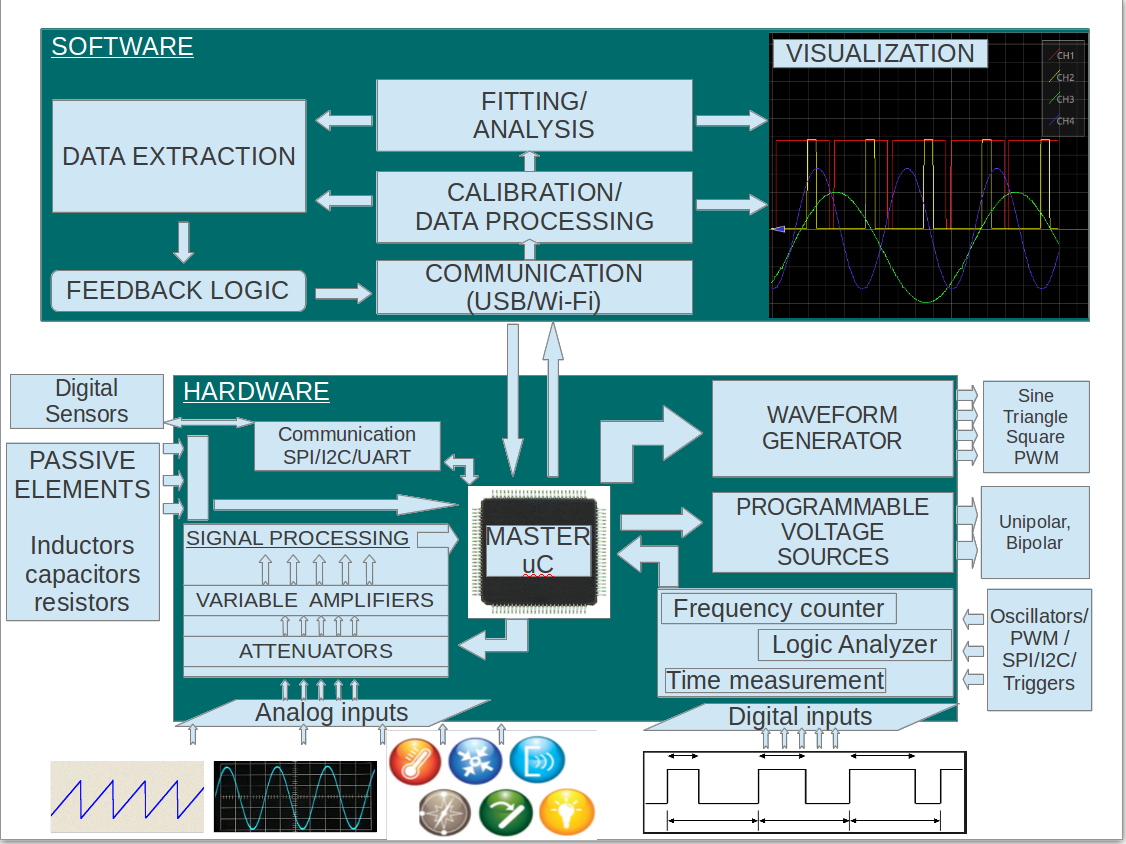
An outline of how this state machine works

But first, you might be interested in the complete set of features of this instrument, and maybe screenshots from a few experiments . Here’s a link to a blog post by Praveen Patil outlining the oscilloscope, controls , and the data logger.

From the flow diagram above, it is apparent that the Hardware communicates to the host PC via a bidirectional communication channel, carries out instructions, and might even communicate to a secondary slave via additional communication channels.

The default state of the PSLab hardware is to listen to the host. The host usually sends a 2- byte header first, the first byte is a broad category classifier, and the second refers to a specific command. Once the header is received , the PSLab either starts executing the task , or listens for further data that may contain configuration parameters

An example for configuring the state of the digital outputs [These values are stored in header files common to the host as well as the hardware:

  • Bytes sent by the host :
    • Byte #1 : 8     #DOUT
    • Byte #2 : 1     #SET_STATE
    • Byte #3 : One byte representing the outputs to be modified, and the nature of the modification (HIGH / LOW ). Four MSB bits contain information regarding the  digital outputs SQR1 to SQR4 that need to be toggled, and four LSBs contain information regarding the state that each selected output needs to be set to.
  • Action taken by the hardware:
    • Move to the set_state routine
    • Set the output state of the relevant output pins (SQR1-4) if required.
    • Respond with an acknowledgement
    • Move back to listening state
  • Bytes Returned by the hardware:
    • Byte #1 : 254 ACKNOWLEDGE. SUCCESSFUL.

In a similar manner, instruments ranging from oscilloscopes, frequency counters, capacitance meters, data buses etc are all handled.

For function calls that are time consuming, the communication process might be split into separate exchanges for initialization, and data download. One such example is the Oscilloscope capture routine. The first information exchange sets the parameters for data acquisition, and the second occurs when the acquisition process is complete.

Host-Side Scripts and Software

The software running on the host runs either a dedicated script that sequentially acquires data or executes control tasks , or it runs an event loop where user inputs are used to determine the acquisition task to be executed.

An example of a pulse sensor designed with just the voltmeter and a digital output of the PSLab.

A photo transistor is connected to the SEN input of the PSLab, and the host software reads the voltage on SEN at fixed intervals.

The conductance of the photo transistor fluctuates along with the incident light intensity, and this is translated into a voltage value by the internal signal processor of the SEN input.

When the photo sensor is covered with a finger, and a bright light is passed through the finger, a time linked plot of these voltage fluctuations reflects the fluctuations in blood pressure, and therefore has the same frequency of the heart beat of the owner of this finger.

* The digital output is used to power a white LED being used as the light source here

Bibliography:

[1] : Original content developed for the SEELablet’s first revision, from which PSLab is derived.

Continue ReadingThe Pocket Science Lab Hardware

Sine Wave Generator

PSLab by FOSSASIA can generate sine waves with arbitrary frequencies. This is very helpful to teachers, students and electronic enthusiasts to study about different frequencies and how systems respond to them. In the device, it uses digital signal processing to derive a smooth sine wave. Except to digital implementation, there are conventional analog implementations to generate a sine wave.

Image from https://betterexplained.com/articles/intuitive-understanding-of-sine-waves/

sine_wave

The most famous method to generate a sine wave is the Wien Bridge Oscillator. It is a frequency selective bridge with a range of arbitrary frequencies. This oscillator has a good stability when it is functioning at its resonance frequency while maintaining a very low signal distortion.           Let’s take a look at this circuit. We can clearly see that there is a series combination of a resistor and a capacitor at A and a parallel combination of a resistor and a capacitor at B joining at the non-inverting pin of the OpAmp. The series combination of RC circuit is nothing but a high pass filter that allows only high frequency components to pass through. The parallel combination of RC circuit is a Low pass filter that allows only the low frequency components of a signal to pass through. Once these two are combined, a band pass filter is created allowing only a specific frequency component to pass through.

It is necessary that the resistor value and the capacitor values should be the same in order to have better performance without any distortion. Assuming that they are same, using complex algebra we can prove that the voltage at V+(3) is one third of the Voltage coming out from the pin (1) of OpAmp.

Using the resonance frequency calculation using RC values, we can determine the frequency of the output sine wave.

f=1/2RC

The combination of two resistors at the inverting pin of the Op Amp controls the gain factor. It is calculated as 1+R1/R2. Since the input to the non-inverting terminal is 1/3 of the output voltage, this gain factor should be maintained at 3. Values greater than 3 will cause a ramping behavior in the sine wave and values below 3 will show an attenuation. So the gain should be set preciously.

Equating 1+R1/R2 to 3, we can obtain a ratio for R1/R2 as 2. That implies R1 should be as twice the resistance of R2. Make sure these resistances are in the power of kilo Ohms. That is to ensure that the leakage current is minimum to the Op Amp. Let’s select R1 = 200K and R2 = 100K

This oscillator supports a range of frequencies. Let’s assume we want to generate a sine wave having 500 Hz. Using f=1/2RC, we can choose arbitrary values for R and C. Substituting values to the formula yields a value for RC = 318 x10e-6

Using practical values for R as 10k, C value can be approximated to 33nF. This oscillator is capable of generating a stable 500 Hz sinusoidal waveform. By changing the resistive and capacitive values of block A and B, we can generate a wide range of frequencies that are supported by the Op Amp because Op Amps have a limited bandwidth it can be functional inside.

It’s worth to note a few facts about generating sine waves using a digital implementation. In analog circuitry, the component values have a tolerance which makes the calculations not perfectly align with the real values. Due to this reason, the actual output will differ from the desired output. In our example to generate 500 Hz sine wave, the capacitors and resistors may have different values and they may have not matched. But with a digital implementation, we can achieve the accuracy and flexibility we require.

External Links:


Continue ReadingSine Wave Generator

Regulating Voltage in PSLab

Electronic components are highly sensitive to voltages and currents across them. Most of the devices in the current market work in the voltage levels of 3.3V, 5V, 12V and 15V. If they are provided with a different voltage than the one required by the vendor, they would not function. If the voltage supplied is higher, they might burn off. The PSLab device requires separate voltage levels such as 3.3V and 5V for its operation.

There are commercial voltage regulators available in the market designed with advanced feedback techniques and models. But we can create out own voltage regulator. In this blog post, I am going to introduce you to a few basic models capable of regulating voltage to a desired level.

Current implementation of PSLab device uses a voltage regulator derived using a zener-resistor combination. This type of regulators have a higher sensitivity to current and their operation may vary when the supplied or the drawn current is lower than the expected values. In order to have a stable voltage regulation, this combination needs to be replaced with a much stable transistor-zener combination.

Before go into much details, let’s get to know a few basic concepts and devices related to.

Zener Diode

Zener DiodeZener diode is a type of diode which has a different operational behavior than the general diode. General diodes allow current to flow only in one direction. If a current in the reverse is applied, they will break and become unusable after a certain voltage level known as Breakdown Voltage. But Zener diodes are specifically designed to function desirably once this break down voltage has been passed and unlike general diode, it can recover back to normal when the voltage is removed or reduced.

Transistor

This is the game changing invention of the 20th century. There are two types of Bipolar Junction Transistors (BJT) available in the market. They are known as NPN and PNP transistors. The difference is based on the polarity of diodes used.

An NPN transistor can be modeled as a combination of two diodes –[NP → PN]– and a PNP transistor can be modeled as –[PN → NP]– using two diodes.

There are three pins to take notice in BJTs. They are illustrated in the diagram shown here;

  1. Base
  2. Collector
  3. Emitter

The amazing fact about BJTs is that the amount of current provided to the Base terminal will control the flow of current going through Collector and Emitter. Also note that always there is a voltage drop across the Base terminal and the Emitter terminal. This typically takes a value of 0.7 V

Voltage Divider

This is the most basic type of voltage regulator. It simply divides the voltage supplied by the battery with the ratio R1:R2. In the following configuration, the output voltage can be calculated using the voltage division rule;

Which is equal to 12 * 100/(100+200) = 4 V

There is a huge drawback with this design. The above calculation is valid only if there is no load impedance is present at the output terminals.

Generally there will be a load impedance and the supplied voltage cannot be easily calculated as the load impedance is unknown to the regulator.

Resistor-Zener Voltage Regulator

Due to the load dependability of the previous model with the load, an improved model can be introduced as follows. This is the current implementation of voltage regulator in PSLab device.

Unlike the previous model, this model ensures that the output voltage will be maintained constant across the output terminals within a range of supply voltage values.

Let’s assume the supply voltage is increased. Then the current flow through the zener diode will increase in order to maintain a constant voltage across the output terminals. In case if the supply voltage drops, then the zener current will decrease and a stable voltage across the output terminals will be maintained.

This design also comes with a slight draw back. This can be explained using the characteristic curve of a zener diode. (Figure is taken from : http://www.electronics-tutorials. ws/diode/diode_7.html)

For a zener diode to maintain a constant voltage level across output terminals, there should be a minimum current flowing through the diode. If this current is not flowing in the zener, there won’t be a regulation. Assume there is a very low load impedance. Then the current supplied by the source will find an easier path to flow other than through the diode. This will affect the regulatory circuit and the desired voltage will not appear across the output terminals.

To compensate the drawback, a much improved design is available using transistors.

Transistor-Zener Voltage Regulator

This is the proposed improvement to the voltage regulatory circuit in PSLab device. In this model, the zener diode is taken away from the load circuit as the current to the load is supplied from the transistor directly. This avoids current limitations to the zener diode had in the previous model and transistor acts as a bridge.

A small current through the Base terminal (1) will support a higher current flow through the output terminal via Collector (2) and Emitter (3). This amplification ratio is in the range of few hundreds for a typical BJT.

A capacitor has been added to compensate ripples from the supply source. If a higher current flow is required through the output terminals, the NPN transistor can be replaced by a Darlington pair.

Using a 5.6 V zener diode and MMBT3904/6 transistors, this model has been implemented in the newest version of PSLab device. They will be supplying a constant voltage of +/- 5V to V+ and V- pins in the device.

External Links:

Continue ReadingRegulating Voltage in PSLab

Constructing and working with Polynomials in the PSLab Android App

PSLab is a device that allows the user to perform a range of science and engineering experiments. PSLab has existing communication library (PSLab Desktop) written in Python. Since we are developing an Android application to operate PSLab, the initial step was to port Python code to JAVA. In PSLab Android application we are using version 3.6.1 of Apache Maths Commons.

NumPy is the package for scientific computing with Python. Polynomials in NumPy can be created using numpy.poly1d. Since some of the files in PSLab Desktop use polynomials, it was important to find a package in JAVA that provides features equivalent to NumPy. Apache Maths Commons fulfilled our needs. It is a Mathematics Library available in JAVA, that provides the means to construct polynomials and perform a range of operations on them. A detailed documentation of the library is available here.

import numpy

p = numpy.poly1d([1, 2, 3])

print(numpy.poly1d(p))

q = p(0.5)

print q

Output:  

1 x2 + 2 x + 3

4.25

Poly1d() function converts a list into polynomials. The first element of the list is the coefficient of the highest degree of the polynomial while the last element is the coefficient of lowest degree of the polynomial. While p(0.5) evaluates polynomial at x = 0.5. 

Now let’s construct polynomials in JAVA using Apache Maths Commons

public class poly {

public static void main(String[] args){

PolynomialFunction p = new PolynomialFunction(new double[]{3, 2, 1});

System.out.println(p);

System.out.println(p.value(0.5));

    }
}

Output:  

3 + 2 x + x^2

4.25

Polynomial Function converts the double array into polynomials. The first element of the array is the coefficient of the lowest degree of the polynomial while the last element is the coefficient of the highest degree of the polynomial. p.value (0.5) evaluates polynomial at x = 0.5.

Other things we can do

  • Find the degree of the polynomial.

Continuing with the above example where polynomial was 3 + 2 x + x^2. p.degree() gives 2 as output which is the degree of the given polynomial.

  • Get the coefficients of the polynomial

p.getCoefficients() returns a double array of the coefficients of the given polynomial. In the above case [3.0, 2.0, 1.0] will be returned.

  • Find derivatives of the polynomial

p.derivative() returns 2 + 2 x which is derivative of polynomial 3 + 2 x + x^2.

  • Add, subtract and multiply two polynomials.

We can add, subtract and multiply 2 polynomials. For example p.multiply(new  Polynomial Function(new double[]{1,2})) returns 3 + 8 x + 5 x^2 + 2 x^3 which is  the product of 3 + 2 x + x^2 and 1 + 2 x

Where are they are used in PSLab?

Polynomials are used in AnalogInputSource.java  to convert raw ADC codes (0=0V , 1023=3.3V ) to voltage values. 

  • calPoly10 = new PolynomialFunction(new double[]{0., 3.3 / 1023, 0.});
  • calPoly12 = new PolynomialFunction(new double[]{0., 3.3 / 4095, 0.});

    Polynomials are also used in DACChannel.java to convert DAC codes to voltage values and vice versa.

  • VToCode = new PolynomialFunction(new double[]{-4095. * intercept / slope, 4095. / slope});                                                    
  • CodeToV = new PolynomialFunction(new double[]{intercept, slope / 4095.});

Continue ReadingConstructing and working with Polynomials in the PSLab Android App

Temporally accurate data acquisition via digital communication pathways in PSLab

This blog post deals with the importance of using a real-time processor for acquiring time dependent data sets. The PSLab already features an oscilloscope, an instrument capable of high speed voltage measurements with accurate timestamps, and it can be used for monitoring various physical parameters such as acceleration and angular velocity as long as there exists a device that can generate a voltage output corresponding to the parameter being measured.  Such devices are called sensors, and a whole variety of these are available commercially.

However, not all sensors provide an analog output that can be input to a regular oscilloscope. Many of the modern sensors use digitally encoded data which has the advantage of data integrity being preserved over long transmission pathways. A commonly used pathway is the I2C data bus, and this blog post will elaborate the challenges faced during continuous data acquisition from a PC, and will explore how a workaround can be managed by moving the complete digital acquisition process to the PSLab hardware in order create a digital equivalent of the analog oscilloscope.

Precise timestamps are essential for extracting waveform parameters such as frequency and phase shifts, which can then be used for calculating physics constants such as the value of acceleration due to gravity, precession, and other resonant phenomena. As mentioned before, oscilloscopes are capable of reliably measuring such data as long as the input signal is an analog voltage, and if a digital signal needs to be recorded, a separate implementation similar to the oscilloscope must be designed for digital communication pathways.

A question for the reader :

Consider a voltmeter capable of making measurements at a maximum rate of one per microsecond.

We would like to set it up to take a thousand readings (n=1000) with a fixed time delay(e.g. 2uS) between each successive sample in order to make it digitize an unknown input waveform. In other words, make ourselves a crude oscilloscope.

Which equipment would you choose to connect this voltmeter to in order to acquire a dataset?

  1. A 3GHz i3 processor powering your favourite operating system, and executing a simple C program that takes n readings in a for loop with a delay_us(2) function call placed inside the loop.
  2. A 10MHz microcontroller , also running a minimal C program that acquires readings in fixed intervals.

To the uninitiated, faster is better, ergo, the GHz range processor trumps the measly microcontroller.

But, we’ve missed a crucial detail here. A regular desktop operating system multitasks between several hundred tasks at a time. Therefore, your little C program might be paused midway in order to respond to a mouse click, or a window resize on any odd chores that the cpu scheduler might feel is more important. The time after which it returns to your program and resumes acquisition is unpredictable, and is most likely of the order of a few milliseconds.

The microcontroller on the other hand, is doing one thing, and one thing only. A delay_us(2) means a 2uS delay with an error margin corresponding to the accuracy of the reference clock used. Simple crystal oscillators usually offer accuracies as good as 30ppm/C, and very low jitter.

Armed with this DIY oscilloscope, we can now proceed to digitize a KHz range since wave or a sound signal from a microphone with good temporal accuracy.

Sample results from the PSLab’s analog oscilloscope

sine wave shown on the oscilloscope
PSLab Oscilloscope showing a 1KHz sinusoidal wave plotted with Matplotlib

If the same were taken via a script that shares CPU time with other processes, the waveform would compress at random intervals due to CPU time unavailability. Starting a new CPU intensive process usually has the effect of the entire waveform appearing compressed because actual time intervals between each sample are greater than the expected time intervals


Implementing the oscilloscope for data buses such as I2C

With regards to the PSLab which already has a reasonably accurate oscilloscope built-in, what happens if one wants to acquire time critical information from sensors connected to the data bus , and not the analog inputs ?

In order acquire such data , the PSLab firmware houses the read routine from I2C in an interrupt function that is invoked at precise intervals by a preconfigured timer’s timeout event. Each sample is stored to an array via a self incrementing pointer.

The I2C address to be accessed, and the bytes to be written before one can start reading data are all pre-configured before the acquisition process starts.

This process then runs at top priority until a preset number of samples have been acquired.Once the host software knows that acquisition should have completed, it fetches the data buffer containing the acquired information.

An example of data being read from a 6-Degree of freedom inertial measurement unit mounted on the pivot of an oscillating physical pendulum.

The plots that overlap accurately with a simulated damped sinusoidal waveform are not possible in the absence of a real-time acquisition system

A 6-DOF sensor connected to the pivot of a physical pendulum.

The sensor in question is the MPU6050 from invensense, used primarily in drones, and other self-stabilising robots.

Its default I2C address is 0x68 ( 104 ) , and 14 registers starting from 0x3B contain data for acceleration along orthogonal axes, temperature, and angular velocity along orthogonal axes. Each of these values is an integer, and is therefore represented by two successive registers. E.g. , 0x3B and 0x3C together make up a 16-bit value for acceleration along the X-axis.


The Final App


Raw Data from a 6-Degree of freedom Inertial Measurement Unit
A least square fit is applied to all 6 datasets (3-axis acceleration, 3-axis angular velocity) from the MPU6050. Extracted parameters show amplitude, frequency, phase and damping coefficient.


Continue ReadingTemporally accurate data acquisition via digital communication pathways in PSLab

Porting PSLab Libraries – Python to Java

PSLab has existing communication libraries and sensor files in Python which were created during the development of Python Desktop Application.

The initial task and challenge was porting this existing code to Java to be used by the Android App. Since, the python libraries also utilized the object oriented model of programming, porting from Python to Java had the similar code structure and organization.

Common problems faced while porting from Python to Java

  • The most common problem is explicitly assigning data types to variables in Java since Python manages data types on its own. However, most of the time the data types are quite evident from the context of their use and understanding the purpose of the code can make the task much simpler.
  • Another task was migrating the Python data structures to their corresponding Java counterparts like a List in Python represents an ArrayList in Java, similarly a Dictionary corresponds to a HashMap and so on.
  • Some of the sections of the code uses highly efficient libraries like Numpy and Scipy for some mathematical functions. Finding their corresponding Java counterparts in libraries was a challenge. This was partly solved by using Apache Common Math which is a library dedicated for mathematical functions. Some of the functions were directly implemented using this library and for rest of the portions, the code was written after understanding the structure and function of Numpy methods.

While porting the code from Python to Java, some of the steps which we followed:

  • Matching corresponding data-structures

The Dictionary in python…

Gain_scaling = OrderedDict ([('GAIN_TWOTHIRDS', 0.1875), ('GAIN_ONE', 0.125), ('GAIN_TWO', 0.0625), ('GAIN_FOUR', 0.03125), ('GAIN_EIGHT', 0.015625), ('GAIN_SIXTEEN', 0.0078125)])

…was mapped to corresponding Java HashMap in the manner given below. A point to be noted here is for adding elements to a HashMap can be done only from a method and not at the time of declaration of HashMap.

private HashMap <String,Double> gainScaling = new HashMap <String,Double>();

gainScaling.put("GAIN_TWOTHIRDS",0.1875);
gainScaling.put("GAIN_ONE",0.125);
gainScaling.put("GAIN_TWO",0.0625);
gainScaling.put("GAIN_FOUR",0.03125);
gainScaling.put("GAIN_EIGHT",0.015625);
gainScaling.put("GAIN_SIXTEEN",0.0078125);

Similarly, the List in Python can be  be converted to the corresponding ArrayList in Java.

  • Assigning data types and access modifiers to corresponding variables in Java
POWER_ON = 0x01
gain_choices = [RES_500mLx, RES_1000mLx, RES_4000mLx]
ain_literal_choices = ['500mLx', '1000mLx', '4000mLx']
scaling = [2, 1, .25]
private int POWER_ON = 0x01;
public int[] gainChoices = {RES_500mLx,RES_1000mLx,RES_4000mLx};
public String[] gainLiteralChoices = {"500mLx", "1000mLx", "4000mLx"};
public double[] scaling = {2,1,0.25};

Assigning data types and the corresponding access modifiers can get tricky sometimes. So, understanding the code is essential to know whether a variable in limited to the class or needs to be accessed outside the class, whether a variable is int, short, float or double etc.

  • Porting Numpy & Scipy functions to Java using Apache Common Math

For example, this piece of code gives the pitch of acceleration. It uses mathematical functions like arc-tan.

pitchAcc = np.arctan2(accData[1], accData[2]) * 180 / np.pi

The corresponding version of arc-tan in Apache Common Math is used in Java.

double pitchAcc = Math.atan2(accelerometerData[1], accelerometerData[2]) * 180 / pi;
  • Porting by writing the code for Numpy and Scipy functions explicitly

In the code below, rfftfreq is used to calculate the Discrete Fourier Transform(DFT) sample frequencies.

freqs = self.fftpack.rfftfreq(N, d=(xReal[1] - xReal[0]) / (2 * np.pi))

Since, hardly any library in Java supports DFT, the corresponding code for rfftfreq was self-written.

double[] rfftFrequency(int n, double space){
    double[] returnArray = new double[n + 1];
    for(int i = 0; i < n + 1; i++){
        returnArray[i] =  Math.floor(i / 2) / (n * space);
    }
    return Arrays.copyOfRange(returnArray, 1, returnArray.length);
}

After porting of all communication libraries and sensor files are done, the testing of features can also be initiated. Currently, the ongoing development includes porting of the some of the remaining files and working on the the best possible User Interface.

Additional Reading

Continue ReadingPorting PSLab Libraries – Python to Java

Integrating Travis CI and Codacy in PSLab Repositories

Continuous Integration Testing and Automated Code Review tools are really useful for developing better software, improving code and overall quality of the project. Continuous integration can help catch bugs by running tests automatically and to merge your code with confidence.

While working on my GsoC-16 project, my mentors guided and helped me to integrate Travis CI and Codacy in PSLab github repositories. This blog post is all about integrating these tools in my github repos, problems faced, errors occurred and the test results.

travisTravis CI is a hosted continuous integration and deployment system. It is used to build and test software projects hosted on github. There are two versions of it, travis-ci.com for private repositories, and travis-ci.org for public repositories.

Read : Getting started with Travis CI

Travis is configured with the “.travis.yml” file in your repository to tell Travis CI what to build. Following is the code from ‘.travis.yml‘ file in our PSLab repository. This repo contains python communication library for PSLab.

language: python
python:
  - "2.6"
  - "2.7"
  - "3.2"
  - "3.3"
  - "3.4"
# - "3.5"
# command to install dependencies
# install: "pip install -r requirements.txt"
# command to run tests
script: nosetests

With this code everything worked out of the box (except few initial builds which errored because of missing ‘requirements.txt‘ file) and build passed successfuly 🙂 🙂

Later Mario Behling added integration to FOSSASIA Slack Channel.

Slack notifications

Travis CI supports notifying  Slack channels about build results. On Slack, set up a new Travis CI integration. Select a channel, and you’ll find the details to paste into your ‘.travis.yml’. Just copy and paste the settings, which already include the proper token and you’re done.

The simplest configuration requires your account name and the token.

notifications:
  slack: '<account>:<token>'     
notifications:
  slack: fossasia:***tokenishidden****

Import errors in Travis builds of PSLab-apps Repository

PSLab-apps repository contains PyQt bases apps for various experiments. The ‘.travis.yml‘ file mentioned above gave several module import errors.

$ python --version
Python 3.2.5
$ pip --version
pip 6.0.7 from /home/travis/virtualenv/python3.2.5/lib/python3.2/site-packages (python 3.2)
Could not locate requirements.txt. Override the install: key in your .travis.yml to install dependencies.
0.33s$ nosetests
E
======================================================================
ERROR: Failure: ImportError (No module named sip)

The repo is installable and PSLab was working fine on popular linux distributions without any errors. I was not able to find the reason for build errors. Even after adding proper ‘requirements.txt‘ file,  travis builds errored.

On exploring the documentation I could figure out the problem.

Travis CI Environment uses separate virtualenv instances for each Python version. System Python is not used and should not be relied on. If you need to install Python packages, do it via pip and not apt. If you decide to use apt anyway, note that Python system packages only include Python 2.7 libraries (default python version). This means that the packages installed from the repositories are not available in other virtualenvs even if you use the –system-site-packages option. Therefore I was getting Import module errors.

This problem was solved by making following changes in the ‘.travis.yml‘ file

language: python

python:
  #- "2.6"
  - "2.7"
  #- "2.7_with_system_site_packages"
  - "3.2"
  #- "3.2_with_system_site_packages"
  - "3.3"
  - "3.4"
before_install:
    - sudo mkdir -p /downloads
    - sudo chmod a+rw /downloads
    - curl -L http://sourceforge.net/projects/pyqt/files/sip/sip-4.16.5/sip-4.16.5.tar.gz -o /downloads/sip.tar.gz 
    - curl -L http://sourceforge.net/projects/pyqt/files/PyQt4/PyQt-4.11.3/PyQt-x11-gpl-4.11.3.tar.gz -o /downloads/pyqt4.tar.gz
    # Builds
    - sudo mkdir -p /builds
    - sudo chmod a+rw /builds

install:
    - export DISPLAY=:99.0
    - sh -e /etc/init.d/xvfb start
    - sudo apt-get install -y libqt4-dev
    - sudo apt-get install -y mesa-common-dev libgl1-mesa-dev libglu1-mesa-dev
#    - sudo apt-get install -y python3-sip python3-sip-dev python3-pyqt4 cmake
    # Qt4
    - pushd /builds
    # SIP
    - tar xzf /downloads/sip.tar.gz --keep-newer-files
    - pushd sip-4.16.5
    - python configure.py
    - make
    - sudo make install
    - popd
    # PyQt4
    - tar xzf /downloads/pyqt4.tar.gz --keep-newer-files
    - pushd PyQt-x11-gpl-4.11.3
    - python configure.py -c --confirm-license --no-designer-plugin -e QtCore -e QtGui -e QtTest
    - make
    - sudo make install
    - popd
 # - "3.5"
# command to install dependencies
#install: "pip install -r requirements.txt"
# command to run tests
script: nosetests

notifications:
  slack: fossasia:*****tokenishidden*******


codacy

Codacy is an automated code analysis and review tool that helps developers ship better software, faster. With Codacy integration one can get static analysis, code complexity, code duplication and code coverage changes in every commit and pull request.

Read : Integrating Codacy in github is here.

Codacy integration has really helped me to understand and enforce code quality standard. Codacy gives you impact of every pull request in terms of quality and errors directly into GitHub.

codacy check

Codacy also grades your project in different categories like Code Complexity, Compatibility, security, code style, error prone etc. to help you better understand the overall project quality and what are the areas you should improve.

Here is a screen-shot of Codacy review for PSLab-apps repository.

codacyreport

I am extremely happy to share that my learning adventure has got  Project Certification at ‘A’ grade. Project quality analysis shows that more than 90% of the work has A grade 🙂 🙂

Travis CI and Codacy Badges for my GSoC Repositories:

PSLab : Python Library for Communication with PSLab

Travis CI Badge         Codacy Badge

PSLab-apps : Qt based GUI applications for PSLab

Travis CI Badge         Codacy Badge

Pocket Science Lab : ExpEYES Programs, Sensor Plugins

Travis CI Badge         Codacy Badge

That’s all for now. Have a happy coding, testing and learning 🙂 🙂

Continue ReadingIntegrating Travis CI and Codacy in PSLab Repositories

Design Your Own Experiments With PSLab

PSLab, with its simple and open architecture allows programmers, hobbyists to use the tool for various measurements and to develop new experiments with simple python code.

One of the main target group, the PSLab is aimed at, is high-school science teachers and students, who may or may-not be familiar with the computer programming. For such users it is difficult to design or develop new experiments on their own. They may also find it difficult to fetch the data and plot required graphs, if a ready-made GUI is not available for that particular experiment.

To enable such users to quickly design a simple experiment for studying various phenomena, we have developed a simple Experiment Designer GUI. This incorporates few controls, read-back elements and easy functions to select parameters and plot graphs.

The screen shot of the ‘Design Your Own Experiment’ GUI along with the App-window is here..

experiment designer1

Experiment Designer allows the user to define the control and read-back sequences of parameters and execute them.

Features of “Design Your Own Experiment” GUI

  • Configure Experiment : Here user can select the required channels ( manual / sweep / read-back). One can also add a derived channel for measuring some physical quantity, for example ‘current’.
  • Make Measurements : Selected channels are displayed. User can make measurements individually for each step or  can sweep in auto mode.
  • Plot and View Plots: Enables user to plot selected parameters. Acquired plots can be selectively displayed or deleted.
  • Save Plots: Data acquired can be save in a spreadsheet.
  • Save Profile : Experiment profile can be saved for repeating the experiment in future. Saved profiles can be loaded from “Load Profile” tab.

Example : Diode IV Characteristics Experiment

For this experiment one needs the following…

  • A variable voltage source : Needs to be swept from Voltage A to  B (say from 0V to 5V)
  • Current Monitoring : Needs to be read for every value of Voltage
  • Plotting and analytics :  Tools to plot the parameters and save data

Schematic Circuit diagram:

diode IV

CH3 monitors the voltage drop across the diode. PV1 is varied in steps, and for each step the current is calculated from the difference between voltages at PV1 and CH3, and the known value of the resistor. For example for 1K resistor, current through the diode is given by

I = (PV1-CH3)/1K

Procedure :

Step 1. Connect Fossasia PSLab to the pc. Connect the components –  Diode from CH3 to Ground and  1k resistor from PV1 to CH3

Step 2. From the terminal Run

Experiments

The App-window will pop-up. Click on ‘Design your own Experiment’ button to get the experiment designer GUI.

experiment designer2

Step 3: Select channels

Sweep Channel PV1 – Sweep from 0.00V -5.00V in 200 steps

Read-back Channel CH3 – for monitoring voltage across the diode

Derived Channel – To measure Current. Type the equation to calculate the current,   (PV1()-CH3())/1000

Step 4. Click on Prepare Experiment‘ to get measurements screen. Click on ‘Evaluate All Rows‘ to make the measurements.

Experiment designer3

Step 5. Select the required columns and click on Plot Selected Columns‘, a message window will pop-up, here user can select the Axes for plotting the graph. On clicking  ‘Plot‘, view plots screen will be displayed.

plotsdiodeiv

One can repeat the experiment and plot multiple curves and save them in a spreadsheet. Acquired plots can be selectively displayed or deleted.

Step 6. The entire design ( Experiment Profile)  of the experiment can be saved for repeating the experiment in future. Saved profiles can be loaded from “Load Profile” tab.

experiment designer profile
This is a very important value add to PSLab Apps. It has enabled PSLab to reach out and help users, who do not have any background in programming. Now ‘designing your own experiments’ has become super easy 🙂 🙂 🙂

Continue ReadingDesign Your Own Experiments With PSLab

PSLab Communication Function Calls

Prerequisite reading:

Interfacing with the hardware of PSLab, fetching the data and plotting it is very simple and straight forward. Various sensors can be connected to PSLab and data can be fetched with a simple python code as shown in the following example…

>>> from PSL import sciencelab
>>> I = sciencelab.connect()     # Initializing: Returns None if device isn't found. The initialization process connects to tty device and loads calibration values.
# An example function that measures voltage present at the specified analog input
>>> print I.get_average_voltage('CH1')
# An example to capture and plot data
>>> I.set_gain('CH1', 3) # set input CH1 to +/-4V range 
>>> I.set_sine1(1000) # generate 1kHz sine wave on output W1 
>>> x,y = I.capture1('CH1', 1000, 10) # digitize CH1 1000 times, with 10 usec interval 
>>> plot(x,y) 
>>> show()
# An example function to get data from magnetometer sensor connected to PSLab
>>> from PSL.SENSORS import HMC5883L #A 3-axis magnetometer >>> M = HMC5883L.connect() >>> Gx,Gy,Gz = M.getRaw() 

The module sciencelab.py contains all the functions required for communicating with PSLab hardware. It also contains some utility functions. The class ScienceLab() contains methods that can be used to interact with the PSLab.

After initiating this class, all the features built into the device can be accessed  using various function calls.


Capture1 : for capturing one trace

capture1(ch, ns, tg)

Arguments

  • ch  : Channel to select as input. [‘CH1′..’CH3′,’SEN’]
  • ns  :  Number of samples to fetch. Maximum 10000
  • tg   :  Time gap between samples in microseconds
#Example >>> x,y = I.capture1('CH1', 1000, 10) # digitize CH1 1000 times, with 10 usec interval

Returns : Arrays X(timestamps),Y(Corresponding Voltage values)


Capture2 : for capturing two traces

capture2(ns, tg, TraceOneRemap='CH1')

Arguments

  • ns :  Number of samples to fetch. Maximum 5000
  • tg  :  Time gap between samples in microseconds
  • TraceOneRemap :   Choose the analogue input for channel 1 (Like MIC OR SEN). It is connected to CH1 by default. Channel 2 always reads CH2.
#Example 
>>> x,y1,y2 = I.capture2(1600,1.75,'CH1') # digitize CH1 and CH2, 1600 times, with 1.75 usec interval

Returns: Arrays X(timestamps),Y1(Voltage at CH1),Y2(Voltage at CH2)


Capture4 : for capturing four taces

capture4(ns, tg, TraceOneRemap='CH1')

Arguments

  • ns:   Number of samples to fetch. Maximum 2500
  • tg :   Time gap between samples in microseconds. Minimum 1.75uS
  • TraceOneRemap :   Choose the analogue input for channel 1 (Like MIC OR SEN). It is connected to CH1 by default. Channel 2 always reads CH2, channel 3 always reads CH3 and MIC is channel 4 (CH4)
#Example
>>> x,y1,y2,y3,y4 = I.capture4(800,1.75) # digitize CH1-CH4, 800 times, with 1.75 usec interval

Returns: Arrays X(timestamps),Y1(Voltage at CH1),Y2(Voltage at CH2),Y3(Voltage at CH3),Y4(Voltage at CH4)


Capture_multiple : for capturing multiple traces

capture_multiple(samples, tg, *args)

Arguments

  • samples:   Number of samples to fetch. Maximum 10000/(total specified channels)
  • tg :   Time gap between samples in microseconds.
  • *args :   channel names
# Example 
>>> from pylab import * 
>>> I=interface.Interface() 
>>> x,y1,y2,y3,y4 = I.capture_multiple(800,1.75,'CH1','CH2','MIC','SEN') 
>>> plot(x,y1) 
>>> plot(x,y2) 
>>> plot(x,y3) 
>>> plot(x,y4) 
>>> show()

Returns: Arrays X(timestamps),Y1,Y2 …


Capture_fullspeed : fetches oscilloscope traces from a single oscilloscope channel at a maximum speed of 2MSPS

capture_fullspeed(chan, amples, tg, *args)

Arguments

  • chan:   channel name ‘CH1’ / ‘CH2’ … ‘SEN’
  • tg :   Time gap between samples in microseconds. minimum 0.5uS
  • *args :   specify if SQR1 must be toggled right before capturing. ‘SET_LOW’ will set it to 0V, ‘SET_HIGH’ will set it to 5V. if no arguments are specified, a regular capture will be executed.
# Example
>>> from pylab import *
>>> I=interface.Interface()
>>> x,y = I.capture_fullspeed('CH1',2000,1)
>>> plot(x,y)               
>>> show()

Returns: timestamp array ,voltage_value array


Set_gain : Set the gain of selected PGA

set_gain(channel, gain)

Arguments

  • channel:   ‘CH1’ , ‘CH2’
  • gain :   (0-7) -> (1x,2x,4x,5x,8x,10x,16x,32x)

Note: The gain value applied to a channel will result in better resolution for small amplitude signals.

# Example
>>> I.set_gain('CH1',7)  #gain set to 32x on CH1


Get_average_voltage : Return the voltage on the selected channel
get_average_voltage(channel_name, **kwargs)
Arguments

  • channel_name:    ‘CH1’,’CH2’,’CH3’, ‘MIC’,’IN1’,’SEN’
  • **kwargs :   Samples to average can be specified. eg. samples=100 will average a hundred readings
# Example 
>>> print I.get_average_voltage('CH4')
1.002

Get_freq : Frequency measurement on IDx. Measures time taken for 16 rising edges of input signal. returns the frequency in Hertz

get_average_voltage(channel='Fin', timeout=0.1)
Arguments

  • channel :    The input to measure frequency from. ‘ID1’ , ‘ID2’, ‘ID3’, ‘ID4’, ‘Fin’
  • timeout :   This is a blocking call which will wait for one full wavelength before returning the calculated frequency. Use the timeout option if you’re unsure of the input signal. returns 0 if timed out
# Example
>>> I.sqr1(4000,25)
>>> print I.get_freq('ID1')
4000.0

Return float: frequency


Get_states : Gets the state of the digital inputs. returns dictionary with keys ‘ID1’,’ID2’,’ID3’,’ID4’
get_states()
#Example
>>> print get_states()
{'ID1': True, 'ID2': True, 'ID3': True, 'ID4': False}

Get_state : Returns the logic level on the specified input (ID1,ID2,ID3, or ID4)
get_state(input_id)
Arguments

  • input_id :    The input channel ‘ID1’ -> state of ID1 ‘ID4’ -> state of ID4
#Example
>>> print I.get_state(I.ID1)
False

Set_state : Set the logic level on digital outputs SQR1,SQR2,SQR3,SQR4
set_state(**kwargs)
Arguments

  • **kwargs :    SQR1,SQR2,SQR3,SQR4 states(0 or 1)
#Example
>>> I.set_state(SQR1=1, SQR2=0) #sets SQR1 HIGH, SQR2 LOw, but leave SQR3,SQR4 untouched.


Continue ReadingPSLab Communication Function Calls

Communicating with Pocket Science Lab via USB and capturing and plotting sine waves

Design of PSLab combines the flexibility of Python programming language and the real-time measurement capability of micro-controllers.

PSLab, with its simple and open architecture allows users to use the tool for various measurements and to develop new experiments with simple functions written in python.

PSLab is interfaced and powered by USB port of the computer. For connecting external signals it has several input/output terminals as shown in the figure.

pslabdesign

Interfacing with the real world

Connecting to PSLab is as simple and straight forward as this…

>>> from PSL import sciencelab
>>> I = sciencelab.connect()     #Returns None if device isn't found
# An example function that measures voltage present at the specified analog input
>>> print I.get_average_voltage('CH1')

Various sensors can be connected to PSLab and data can be fetched with a simple python code as shown below…

>>> from PSL.SENSORS import HMC5883L #A 3-axis magnetometer
>>> M = HMC5883L.connect()
>>> Gx,Gy,Gz = M.getRaw()

The module sciencelab.py contains all the functions required for communicating with PSLab hardware. It also contains some utility functions. The class ScienceLab() contains methods that can be used to interact with the PSLab. The connect() function returns an object of this class if PSLab hardware is detected.

The initialization process does the following

* connects to tty device

* loads calibration values.

>>> from PSL import sciencelab
>>> I = sciencelab.connect()
>>> print I
<PSL.sciencelab.ScienceLab instance at 0x7fe9a7bf0e18>

After initiating this class, its various function calls will allow access to all the features built into the device. Some examples showing the use of few function calls are given below…

Example 1: Capturing and plotting a sine wave

The function call used,

capture1(self,ch,ns,tg,*args,**kwargs)

Arguments

  • ch  : Channel to select as input. [‘CH1′..’CH3′,’SEN’]
  • ns  :  Number of samples to fetch. Maximum 10000
  • tg   :  Time gap between samples in microseconds

Example Program

Connect WG1 to CH1 and run the following code.

>>> from pylab import *
>>> from PSL import sciencelab
>>> I=sciencelab.connect()
>>> I.set_gain('CH1', 3) # set input CH1 to +/-4V range
>>> I.set_sine1(1000) # generate 1kHz sine wave on output W1
>>> x,y = I.capture1('CH1', 1000, 10) # digitize CH1 1000 times, with 10 usec interval
>>> plot(x,y)
>>> show()

For running the script in IDE, one should define source code encoding, add this to the top of your script:

# -*- coding: utf-8 -*-

The output of the program is here…

sine1

Example 2 : Capturing two sine waves and plotting

The function call used,

capture2(self,ns,tg,TraceOneRemap='CH1')

Arguments

  • ns :  Number of samples to fetch. Maximum 5000
  • tg  :  Time gap between samples in microseconds
  • TraceOneRemap :   Choose the analogue input for channel 1 (Like MIC OR SEN). It is connected to CH1 by default. Channel 2 always reads CH2.

Example Program

Connect WG1 to CH1, WG2 to CH2 and run the following code.

# -*- coding: utf-8 -*-

from pylab import *
from PSL import sciencelab
I=sciencelab.connect()
I.set_gain('CH1', 2) # set input CH1 to +/-4V range
I.set_gain('CH2', 3) # set input CH2 to +/-4V range
I.set_sine1(1000) # generate 1kHz sine wave on output W1
I.set_sine2(1000) # generate 1kHz sine wave on output W2

x,y1,y2 = I.capture2(1600,1.75,'CH1') 
plot(x,y1) #Plot of analog input CH1
plot(x,y2) #plot of analog input CH2
show()

The output of the program is here…sine2

Example 3 : Capturing four traces and plotting

The function call used,

capture4(self,ns,tg,TraceOneRemap='CH1')

Arguments

  • ns:   Number of samples to fetch. Maximum 2500
  • tg :   Time gap between samples in microseconds. Minimum 1.75uS
  • TraceOneRemap :   Choose the analogue input for channel 1 (Like MIC OR SEN). It is connected to CH1 by default. Channel 2 always reads CH2.

Example Program

Connect WG1 to CH1, WG2 to CH2, SQR1 to CH3 and transducer mic to MIC (CH4) and run the following code.

# -*- coding: utf-8 -*-

from pylab import *
from PSL import sciencelab
I=sciencelab.connect()
I.set_gain('CH1', 2) # set input CH1 to +/-4V range
I.set_gain('CH2', 3) # set input CH2 to +/-4V range
I.set_sine1(1000) # generate 1kHz sine wave on output W1
I.set_sine2(1000) # generate 1kHz sine wave on output W2
I.sqr1(2000,duty_cycle=50) # generate 1kHz square wave on output SQR1

x,y1,y2,y3,y4 = I.capture4(800,1.75)
plot(x,y1) #Plot of analog input CH1
plot(x,y2) #plot of analog input CH2
plot(x,y3) #plot of analog input CH3
plot(x,y4) #plot of analog input CH4 : MIC
show()

The output of the program is here…waves

Next To Do for GSoC-16

A detailed User manual and programmers manual with description of all function calls. ( Work in progress 🙂  )

Read:
  1. Post about installing PSLab
  2. PSLab and ExpEYES and GSoC-16 work
Continue ReadingCommunicating with Pocket Science Lab via USB and capturing and plotting sine waves